If you want to pull a subset of rows from a list based on one or more conditions, the FILTER function in Excel is the cleanest way to do it.
FILTER is a dynamic array function. It spills its results across the cells below, and the output updates automatically when your data changes.
In this article, I’ll walk you through how to use FILTER with single and multiple conditions, handle no-match cases, do partial text matches, and combine it with SORT.
FILTER Function Syntax in Excel
The FILTER function returns a filtered subset of an array based on a Boolean condition. Here’s the syntax:
=FILTER(array, include, [if_empty])
- array (required): The range or array you want to filter.
- include (required): A Boolean array, the same height or width as
array, that tells FILTER which rows or columns to keep. - if_empty (optional): The value to return when no rows match. If you skip it and nothing matches, FILTER returns a #CALC! error.
When to Use FILTER Function
- You want to extract rows from a table that match one or more conditions.
- You need the filtered output to update automatically as the source data changes.
- You want to chain a filter with other dynamic array functions like SORT or UNIQUE.
- You want a formula-based filter instead of Excel’s built-in filter dropdowns, which don’t update on data changes.
- You want to return only specific rows based on a partial text match or a calculated condition.
Example 1: Filter Rows That Match a Single Value
Let’s start with a simple example.
Below is the dataset of employees, their departments, and salaries.
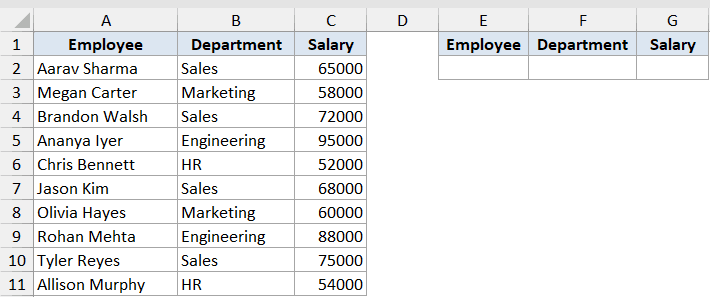
We want to pull out every employee who works in the Sales department.
Here is the formula:
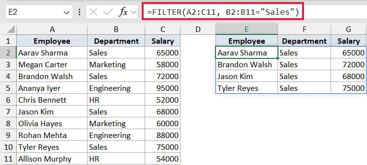
=FILTER(A2:C11, B2:B11="Sales")
How this formula works:
- array is
A2:C11, the full employee table including the Employee, Department, and Salary columns. - include is
B2:B11="Sales", a Boolean array where TRUE marks every row where Department equals “Sales”. - FILTER keeps the rows where the Boolean is TRUE and spills them into the cells starting at E2.
Notice that you only enter the formula in E2. The four matching rows spill into the cells below and to the right on their own.
Pro Tip: The FILTER output is a single spill range. If you add a new Sales employee to the source table, the result updates automatically and the spill expands by one row.
Example 2: Use if_empty to Handle No-Match Cases
Here’s a practical scenario.
Below is a list of orders with their statuses and amounts.
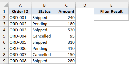
We want to pull every order with status “Refunded”. But there are no refunded orders in this list, so we want the formula to return a clean message instead of a #CALC! error.
Here is the formula:
=FILTER(A2:C9, B2:B9="Refunded", "No matching orders")
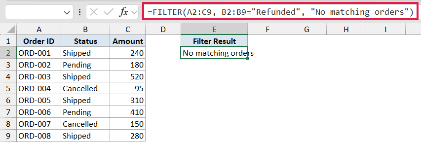
The third argument, if_empty, kicks in only when the Boolean array has no TRUE values. Here, since no row has Status equal to “Refunded”, FILTER returns the string “No matching orders” in cell E2.
Without the third argument, the same formula would return a #CALC! error, which looks broken on a worksheet you’re sharing.
Pro Tip: You can return an empty string (“”) for if_empty if you don’t want anything visible when there’s no match. That’s useful when the FILTER output feeds into another formula that breaks on text.
Example 3: Filter With Multiple AND Criteria
Let’s step it up.
Below is a dataset of sales reps with their region and sales numbers.
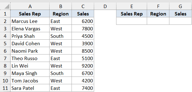
We want to pull every rep who is in the West region AND has sales above 5000.
Here is the formula:
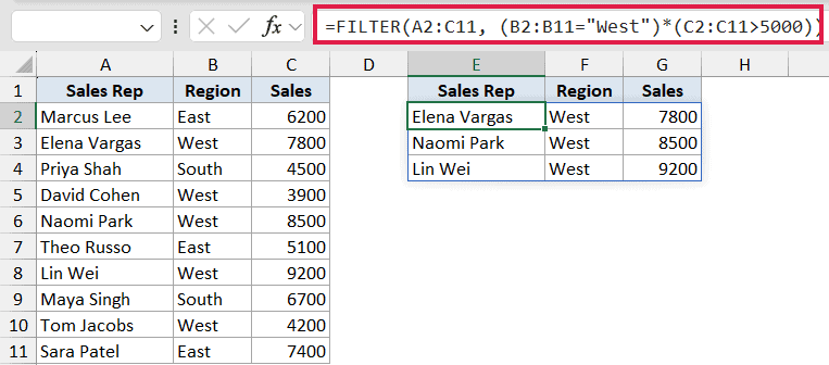
=FILTER(A2:C11, (B2:B11="West")*(C2:C11>5000))
How this formula works:
- Each condition
B2:B11="West"andC2:C11>5000returns a Boolean array of TRUE/FALSE values. - Multiplying the two arrays together gives a combined array where the value is 1 only when both conditions are TRUE (1 × 1 = 1). If either is FALSE (0), the product is 0.
- FILTER treats 1 as TRUE and 0 as FALSE, so only rows where both are true are kept.
The * operator is how you build an AND condition inside FILTER. You can stack as many conditions as you need by multiplying more Boolean arrays into the include argument.
Example 4: Filter With Multiple OR Criteria
Now let’s flip the logic to OR.
Below is a list of students with the subject they’re enrolled in and their score.
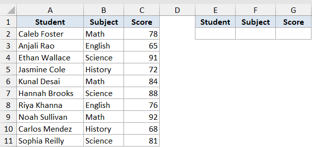
We want to pull every student who is taking Math OR Science.
Here is the formula:
=FILTER(A2:C11, (B2:B11="Math")+(B2:B11="Science"))
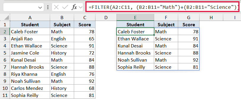
For OR logic, use the + operator. Each condition is still a Boolean array, but adding them together gives a value of 1 if either condition is TRUE (or 2 if both are, which FILTER still treats as TRUE).
Six rows match (three Math students plus three Science students), and they all spill into the output range starting at E2.
Pro Tip: When a row matches more than one condition with `+`, the include value becomes 2 instead of 1. FILTER still keeps the row (it treats any non-zero value as TRUE), so duplicates are not a problem.
Example 5: Filter With a Partial Text Match
Here’s a common gotcha.
FILTER does not support wildcards like * or ? directly. So if you want to find rows where a column contains a substring (like an email containing “gmail”), you have to combine FILTER with ISNUMBER and SEARCH.
Below is a list of customers with their email and city.
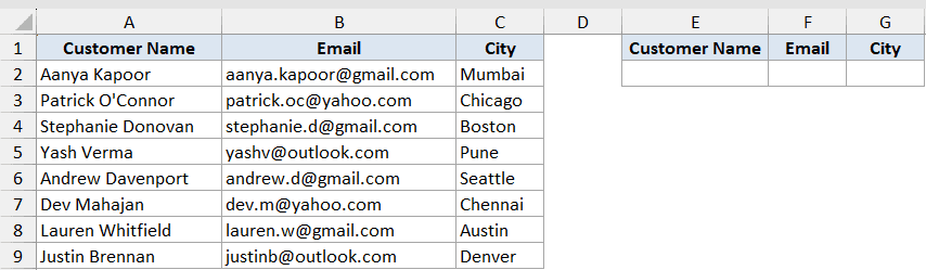
We want to filter only the customers whose email contains the text “gmail”.
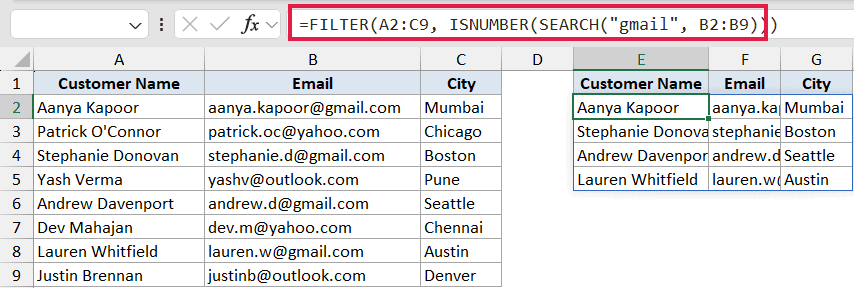
Here is the formula:
=FILTER(A2:C9, ISNUMBER(SEARCH("gmail", B2:B9)))
How this formula works:
SEARCH("gmail", B2:B9)looks for “gmail” inside each email and returns the position number if found, or a #VALUE! error if not.ISNUMBER(...)converts that into a clean TRUE/FALSE array. Position numbers become TRUE, errors become FALSE.- FILTER uses that Boolean array to keep only the matching rows.
This is the standard pattern for “contains” matches inside FILTER. SEARCH is case-insensitive; swap it for FIND if you need case-sensitive matching.
Example 6: Combine FILTER With SORT
For the last one, let’s do filtering and sorting in a single formula.
Below is a dataset of employees, their department, and their salary.
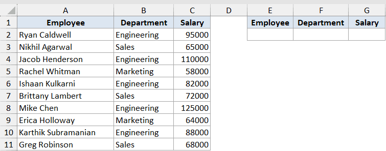
We want to pull only the Engineering employees and sort them by salary in descending order, all in one formula.
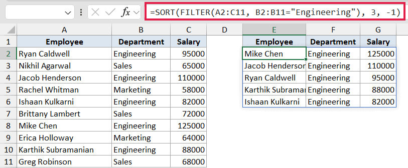
Here is the formula:
=SORT(FILTER(A2:C11, B2:B11="Engineering"), 3, -1)
How this formula works:
- The inner FILTER pulls every row where Department equals “Engineering”.
- SORT then takes that filtered array, sorts it by the third column (Salary), with
-1meaning descending order. - The result spills into the cells below E2, fully sorted and fully filtered in one step.
This is the kind of composition dynamic arrays make easy. You can chain UNIQUE, SORT, FILTER, and SEQUENCE together without wrapping them in CSE braces or pressing Ctrl+Shift+Enter.
Tips & Common Mistakes
- Use
*for AND and+for OR. Don’t try to nest AND() or OR() inside FILTER’s include argument. Those functions return a single TRUE/FALSE and break the array logic. Always combine Boolean arrays with multiplication or addition. - Always include the third argument when there’s any chance of a no-match result. A bare FILTER that returns nothing throws #CALC!. The
if_emptyargument is the cleanest way to handle this. - Watch for #SPILL! errors. FILTER needs empty cells to spill into. If any cell in the destination range already has a value, you’ll see #SPILL! until you clear the blocking cells.
- FILTER does not do wildcards. No
*or?support. Use ISNUMBER + SEARCH for “contains” matches, or LEFT / RIGHT comparisons for “starts with” / “ends with”. - The Boolean array must match the dimensions of
array. IfarrayisA2:C11(10 rows),includemust also be 10 rows. A mismatch returns #VALUE!. - Make sure your Excel version supports FILTER. It’s available in Excel 365, Excel 2021, and Excel for the Web. It does not work in Excel 2019 or earlier.
Before FILTER existed, pulling rows by condition meant SUMPRODUCT, AGGREGATE, or CSE array formulas. FILTER does the same job in a single line, and the result updates automatically as your data changes.
Once you’re comfortable with the AND, OR, and “contains” patterns above, you can build pretty much any extract-rows-by-condition formula in a single line.
Related Excel Functions / Articles: