If you have the year, month, and day sitting in separate cells and you want Excel to treat them as one real date, the DATE function is what you need. It takes three numbers and returns a proper Excel date you can sort, filter, and calculate with.
In Excel 365, you can also feed DATE whole ranges, and the results spill into the cells below in one shot. In this article, I’ll walk you through how DATE works with six practical examples.
DATE Function Syntax in Excel
The DATE function builds a date from three separate values.
=DATE(year,month,day)
- year – the year for the date. Always use a four-digit year like 2025. Two-digit years are read in a way that’s easy to misjudge, so avoid them.
- month – the month number, from 1 to 12. Numbers outside that range roll over into the next or previous year.
- day – the day number. Numbers outside the normal range for that month roll into the next or previous month.
When to Use DATE Function
Here are the most common situations where DATE earns its keep:
- You have year, month, and day in separate columns and need to combine them into a real date.
- You want to build a date that doesn’t depend on regional settings, so it reads the same on every machine.
- You need a hard date boundary to feed into functions like SUMIFS, COUNTIFS, or FILTER.
- You want to shift a date forward or back by a set number of years or months.
Example 1: Combine Year, Month, and Day
Let’s start with the most common job DATE does.
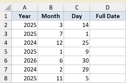
Below is the dataset. It has the year, month, and day for each record split across three columns, with an empty Full Date column waiting to be filled.
I want to pull the three numbers in each row together into one real date in column D.
Here is the formula:
=DATE(A2:A8,B2:B8,C2:C8)
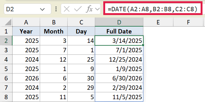
Because I passed whole ranges instead of single cells, this one formula in D2 spills down through D8 on its own. The first result is March 14, 2025, and every row below fills automatically.
There’s no need to copy the formula down. If you add more rows to the source data, just widen the ranges and the spill grows with them. This is one of several ways to insert a date in Excel, and it’s the cleanest when your parts live in separate columns.
Pro Tip: If you’re on an older version of Excel without spill support, write =DATE(A2,B2,C2) in D2 and copy it down. Same result, one cell at a time.
Example 2: Out-of-Range Months and Days
Here’s something about DATE that trips people up at first.
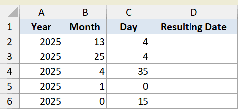
Below is the dataset. The Month and Day columns hold some deliberately out-of-range values, like month 13, day 35, and a couple of zeros.
I want to see what DATE actually returns when the inputs go past their normal limits.
Here is the formula:
=DATE(A2,B2,C2)
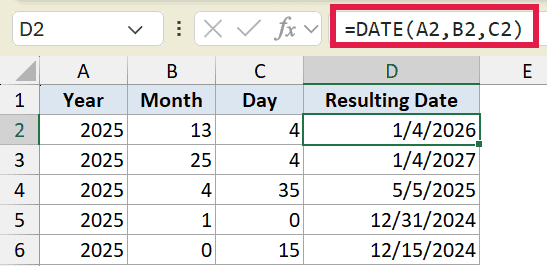
DATE doesn’t throw an error. It rolls the overflow over. Month 13 of 2025 becomes January 2026, so the first row returns January 4, 2026.
The same logic applies to days. A day of 35 pushes into the next month, and a day of 0 lands on the last day of the previous month. A month of 0 rolls back to December of the prior year.
This rollover behavior is handy on purpose. You can write =DATE(2025,13,1) to mean “the first day after December 2025” without doing the math yourself.
Example 3: Add Years to a Date
Now let’s use DATE to shift a date by a fixed number of years.
Below is the dataset. Column A has a few start dates, and I want to work out the five-year anniversary of each one in column B.
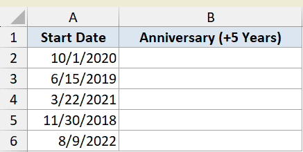
I want each anniversary date to keep the same month and day, but land five years later.
Here is the formula:
=DATE(YEAR(A2)+5,MONTH(A2),DAY(A2))
The trick here is pulling apart the original date with YEAR, MONTH, and DAY, then rebuilding it with five added to the year. The first row, October 1, 2020, becomes October 1, 2025. There are a few other ways to add years to a date in Excel if you want to compare approaches.
Pro Tip: For shifting a date by whole months or years, the EDATE function is more direct: =EDATE(A2,60) adds 60 months (five years). The DATE rebuild still works everywhere, including older Excel, so it’s worth knowing both.
Example 4: Add Months to a Date
Adding months works the same way, with one wrinkle worth watching. If you want a deeper look at this, see the full guide on how to add months to a date in Excel.
Below is the dataset. Column A has invoice dates, and I want a due date two months out for each one in column B.
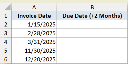
I want each due date to sit exactly two months after the invoice date.
Here is the formula:
=DATE(YEAR(A2),MONTH(A2)+2,DAY(A2))
I add 2 to the month and let DATE handle the rollover. The first invoice, January 15, 2025, gets a due date of March 15, 2025.
Watch the last two rows. November 30 plus two months and December 20 plus two months both cross into 2026, since adding to the month rolls the year forward when it goes past 12.
Example 5: Build Date Boundaries for SUMIFS
DATE is at its most useful when you need a hard date boundary to feed another function. This is where it beats typing a date as text.
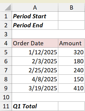
Below is the layout. The top two cells hold a period start and end, then there’s a small table of orders, and a Q1 Total cell at the bottom.
First I’ll set the start of the period in B1.
Here is the formula:
=DATE(2025,1,1)
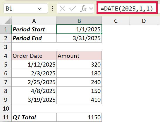
This gives a clean January 1, 2025, no matter what date format the machine uses. Now I’ll set the end of the period in B2.
Here is the formula:
=DATE(2025,3,31)
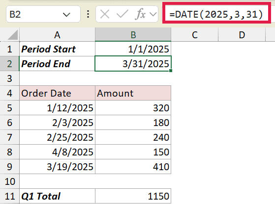
That’s March 31, 2025, the last day of Q1. With both boundaries in place, I can total only the orders that fall inside the quarter.
Here is the formula:
=SUMIFS(B5:B9,A5:A9,">="&DATE(2025,1,1),A5:A9,"<="&DATE(2025,3,31))
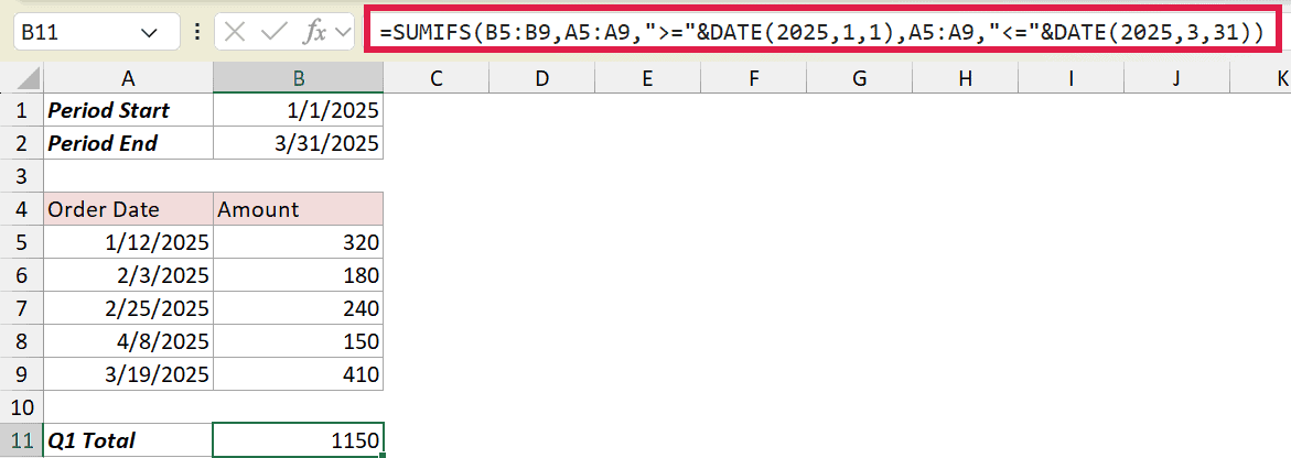
The total comes to 1150. The April 8 order is left out because it falls past the March 31 boundary. If you want the full rundown on the SUMIFS function, it’s worth a read.
Building the boundaries with DATE instead of "1/1/2025" keeps the formula safe across regions. A text date like that can be read as January 1 or as the first of an entirely different month depending on local settings.
Example 6: Pull Records Between Two Dates with FILTER
For the last example, let’s use DATE boundaries to pull the actual rows that fall inside a date range, not just a total.
Below is the dataset. It lists six orders with their region, order date, and amount. There’s also a header, Orders from Q1 2025, sitting off to the right in column E where the results will go.
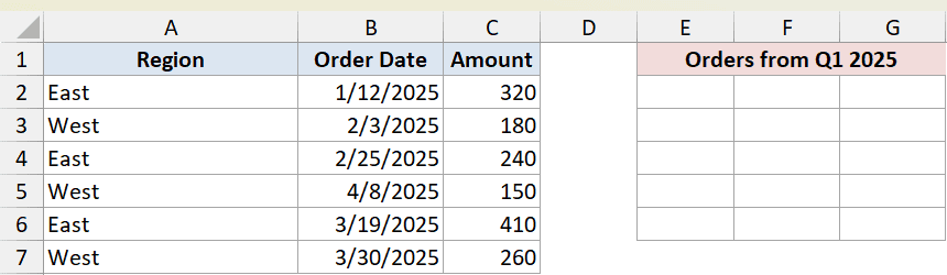
I want to pull every order placed in Q1 2025, the full row, not just a count.
Here is the formula:
=FILTER(A2:C7,(B2:B7>=DATE(2025,1,1))*(B2:B7<=DATE(2025,3,31)))
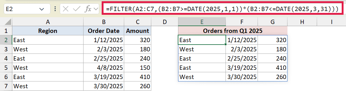
The matching rows spill underneath the Orders from Q1 2025 header, starting at E2. Five of the six orders qualify, and the April 8 order drops out because it sits past the March 31 boundary.
The two DATE calls set the start and end of the quarter, and multiplying the two conditions together keeps only the rows that satisfy both. FILTER then returns those rows as a spilled range.
Pro Tip: Use SUMIFS when you want a single number for the date range, and FILTER when you want to see the matching rows themselves. DATE builds the boundaries for both.
Tips & Common Mistakes
- Always use four-digit years. A value like 25 gets interpreted in a way that’s easy to get wrong, while 2025 is never ambiguous.
- Don’t type dates as plain text when you can build them with DATE. Text dates depend on regional settings, so the same string can mean different things on different machines.
- Out-of-range months and days roll over instead of erroring. That’s useful once you know it, but it can hide a typo, so sanity-check your inputs.
- To shift a date by whole months or years, EDATE is shorter than rebuilding with DATE. Reach for DATE when you need full control over all three parts or when you’re stuck on older Excel.
- In Excel 365, feed DATE a range and let it spill rather than copying a single-cell formula down.
DATE is one of those small functions you end up using all the time once it clicks. It turns loose numbers into real dates, shifts dates around by years or months, and hands you locale-proof boundaries for the likes of SUMIFS, COUNTIFS, and FILTER.
Keep four-digit years in mind, remember the rollover behavior, and you’ll rarely fight with dates in Excel again.
Related Excel Functions / Articles:
- EOMONTH Function in Excel
- TODAY Function in Excel
- DATEDIF Function in Excel
- Get End of Year Date in Excel (Formula)
- How to Add Days to a Date in Excel
- How to Convert Date to Month and Year in Excel
- How to Remove Year from Date in Excel?
- Using IF Function with Dates in Excel (Easy Examples)
- How to Convert Serial Numbers to Date in Excel