If you want to find the position of a value in a list or a row, the XMATCH function is what you’re looking for. It’s the modern successor to MATCH, and it does the same job with less fuss.
XMATCH is a dynamic array function. Feed it an array of lookup values and it spills a whole column or row of positions in one formula.
In this article, I’ll show you how to use XMATCH for exact matches, reverse searches, approximate matches, wildcard matches, and two-way lookups.
XMATCH Function Syntax in Excel
Here is the syntax of the XMATCH function:
=XMATCH(lookup_value,lookup_array,[match_mode],[search_mode])
- lookup_value – the value you want to find. This can be a single value or an array of values.
- lookup_array – the row or column you want to search.
- match_mode – optional. How the value is matched:
– 0 – exact match (this is the default). – -1 – exact match, or the next smaller value if no exact match is found. – 1 – exact match, or the next larger value if no exact match is found. – 2 – wildcard match, where *, ?, and ~ are treated as wildcards.
- search_mode – optional. The direction of the search:
– 1 – search first to last (this is the default). – -1 – search last to first, which returns the last match. – 2 – binary search on data sorted in ascending order. – -2 – binary search on data sorted in descending order.
XMATCH returns the relative position within the lookup_array. Position 1 is the first cell of the array, not the worksheet row it sits in.
When to Use XMATCH Function
Here are some common situations where XMATCH comes in handy:
- When you want the position of a value in a list, so you can feed it into INDEX or another function.
- When you need the last occurrence of a value instead of the first.
- When you want the nearest tier in a banded table, like a shipping rate or a tax bracket.
- When you want to match partial text using wildcards.
- When you want a flexible two-way lookup without VLOOKUP’s column-counting.
Example 1: Find the Position of a Value
Let’s start with the most basic use of XMATCH.
Below is the dataset with sales reps in column A and their Q1 sales in column B. Below the data is a small input area where the rep to look up sits in cell B9.
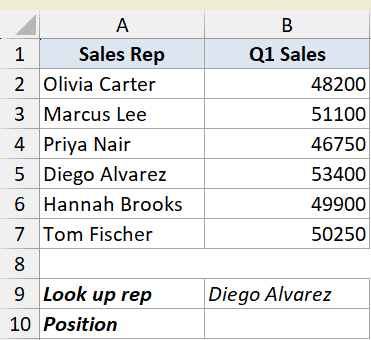
I want to find the position of “Diego Alvarez” within the list of reps in A2:A7.
Here is the formula:
=XMATCH(B9,A2:A7)
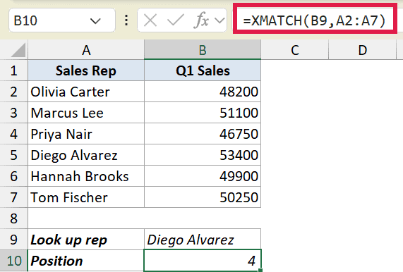
The formula returns 4, because Diego Alvarez is the fourth name in the list.
Notice there’s no third argument. Exact match is the default in XMATCH, so you don’t need to add the 0 that MATCH always asked for.
Pro Tip: The position is relative to the lookup_array, not the worksheet. Diego is in worksheet row 5, but XMATCH returns 4 because he’s the fourth cell in A2:A7.
Example 2: Spill Positions for a List of Values
Here’s where XMATCH pulls ahead of MATCH.
Below is the same rep list, with three reps to find in A10:A12. We want a position for each one.
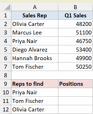
Instead of writing one formula per rep, I’ll feed the whole range A10:A12 in as the lookup value.
Here is the formula:
=XMATCH(A10:A12,A2:A7,0)
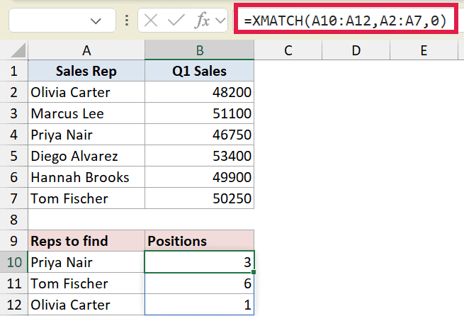
One formula in B10 spills three results down the column: 3, 6, and 1. Each number is the position of the matching rep in A2:A7.
This is the dynamic array behavior. You write the formula once, and the results fill the cells below automatically. Just make sure those cells are empty, or you’ll get a #SPILL! error.
Example 3: Find the Last Match With Reverse Search
Sometimes the first match isn’t the one you want. You want the most recent one.
Below is an order log where “Marcus Lee” appears three times, in rows 2, 4, and 6.
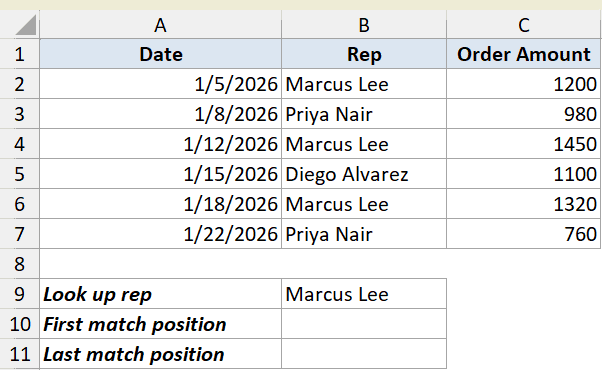
First, let’s find the position of his first order using the default search direction.
Here is the formula:
=XMATCH(B9,B2:B7,0,1)
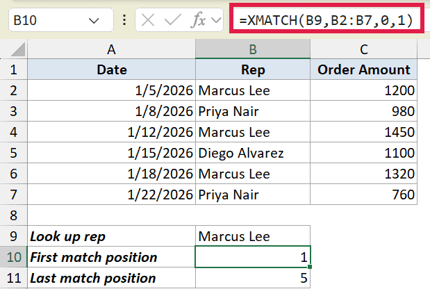
This returns 1, because Marcus Lee’s first order is the first row in B2:B7. The fourth argument 1 tells XMATCH to search first to last.
Now let’s find his last order by flipping the search direction.
Here is the formula:
=XMATCH(B9,B2:B7,0,-1)
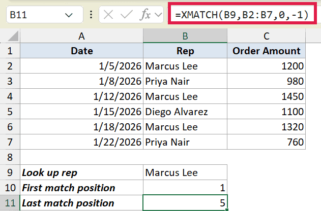
This returns 5. The -1 search mode makes XMATCH search last to first, so it lands on his most recent order in position 5.
This is something MATCH can’t do without array tricks. XMATCH handles reverse search with a single argument.
Example 4: Approximate Match (Next Smaller and Next Larger)
XMATCH can also find the nearest value when there’s no exact match.
Below is a shipping-rate table. Each row gives the minimum weight for a tier, and we have a package that weighs 13 kg in cell B8.
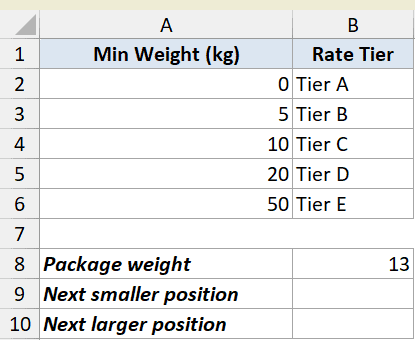
There’s no row for exactly 13 kg, so first let’s find the next smaller weight using match_mode -1.
Here is the formula:
=XMATCH(B8,A2:A6,-1)
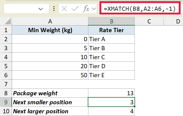
This returns 3. The next value at or below 13 is 10, which sits in position 3 (Tier C).
Now let’s find the next larger weight using match_mode 1.
Here is the formula:
=XMATCH(B8,A2:A6,1)
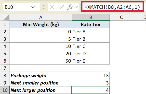
This returns 4. The next value at or above 13 is 20, which sits in position 4 (Tier D).
Pro Tip: Unlike MATCH, XMATCH does not force you to sort the lookup array in a specific direction for approximate matches. That alone removes one of the most common MATCH errors.
Example 5: Wildcard Match for Partial Text
You can also match on a partial text pattern with XMATCH.
Below is a list of product codes. We want to find the first code that starts with “BX-“, so the search pattern in B8 is BX-*.
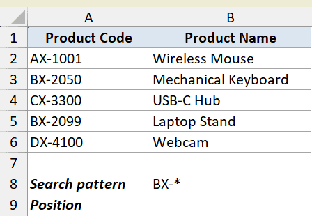
To make the asterisk work as a wildcard, I’ll set match_mode to 2.
Here is the formula:
=XMATCH(B8,A2:A6,2)
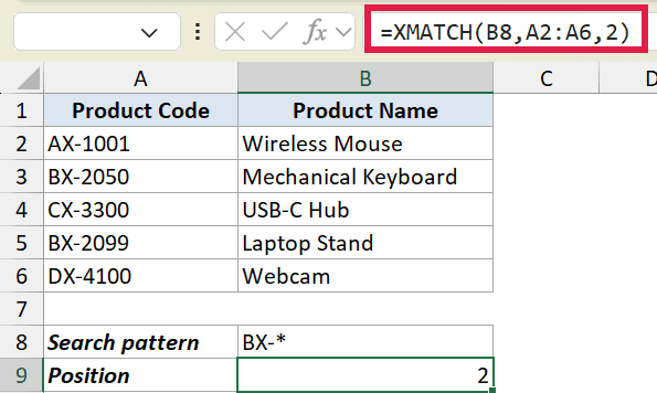
This returns 2, the position of “BX-2050”, the first code that matches the pattern.
The * stands for any number of characters. With match_mode 2, you can also use ? for a single character, and ~ to escape a literal wildcard. The same idea works with wildcard in XLOOKUP when you also need to return a value.
Example 6: Two-Way Lookup With INDEX and XMATCH
For the last example, let’s pull a value from the intersection of a row and a column.
Below is a headcount table with departments down the side and months across the top. We want the headcount for Engineering in February.
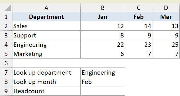
I’ll use the INDEX function for the lookup, with one XMATCH for the row position and another for the column position.
Here is the formula:
=INDEX(B2:D5,XMATCH(B7,A2:A5),XMATCH(B8,B1:D1))
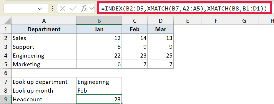
This returns 23, the headcount where Engineering and Feb meet.
Here is how this formula works:
- The first XMATCH finds “Engineering” in A2:A5 and returns 3 (the row position).
- The second XMATCH finds “Feb” in B1:D1 and returns 2 (the column position).
- INDEX then returns the value at row 3, column 2 of B2:D5, which is 23.
This is cleaner than VLOOKUP because you never count columns by hand, and either lookup can change without breaking the formula. If you’d rather skip INDEX entirely, the XLOOKUP function does two-way lookups on its own.
Tips & Common Mistakes
- XMATCH returns a relative position, not a worksheet row. Position 1 is the first cell of the lookup_array. If your array starts in row 2, add an offset only when you actually need to find the row number of matching value.
- XMATCH needs Excel 365 or Excel 2021 and later. It won’t appear in older versions. For Excel 2019 and earlier, use the MATCH function, which is the legacy equivalent.
- Don’t add
0out of habit. Exact match is the default, so you can drop the match_mode argument entirely for an exact match. - Watch for
#SPILL!errors. When you feed XMATCH an array of lookup values, keep the cells below the formula empty so the results have room to spill. - No sorting needed for approximate matches. MATCH demands a sorted array, but XMATCH does not, which saves you from a frequent source of wrong results.
XMATCH does everything MATCH does, then adds exact match by default, reverse search, sort-free approximate matches, and wildcards. Pair it with INDEX and you can look up values in any direction.
If you’re on Excel 365 or 2021, there’s not much reason to keep using MATCH.
Related Excel Functions / Articles: