How to Use VLOOKUP with Multiple Criteria in Excel

If you’ve ever tried to look up a value that depends on more than one condition, you’ve hit VLOOKUP’s biggest limitation.

It only matches one lookup value against one column. So “find the salary for the Finance department AND the Evening shift” isn’t something it does on its own.

The good news is there are several dependable ways around it, and a couple of them are far cleaner than the classic workaround.

In this tutorial I’ll show you six of them. The first two are real VLOOKUP methods, so those are the ones to use if you’re tied to VLOOKUP.

The other four swap VLOOKUP out for a different function that handles multiple criteria on its own. I’ll say which is which as we go.

I’ll also cover what to do when two criteria aren’t enough and when your criteria live on another sheet.

Method #1: Using a Helper Column and VLOOKUP

The simplest fix is to give VLOOKUP the single column it wants. You join your two criteria into one helper column, then look that combined value up.

I reach for this method first when I’m teaching someone, because you can see the combined key sitting right there in the sheet.

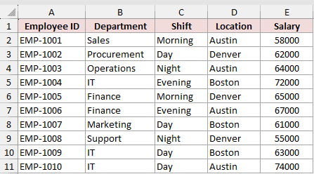
Below I have an employee roster with the Employee ID, Department, Shift, Location, and Salary. I want to pull the salary for a specific department and shift combination, in this case Finance and Evening.

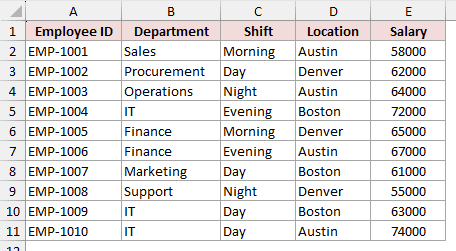
Start by inserting a helper column to the left of the data, so it becomes the new column A. In cell A2, join the department and shift with a delimiter:

=C2&"|"&D2

Copy this down the column. For the Finance Evening row it returns Finance|Evening. The | character is just a separator that keeps the two pieces from blurring together.

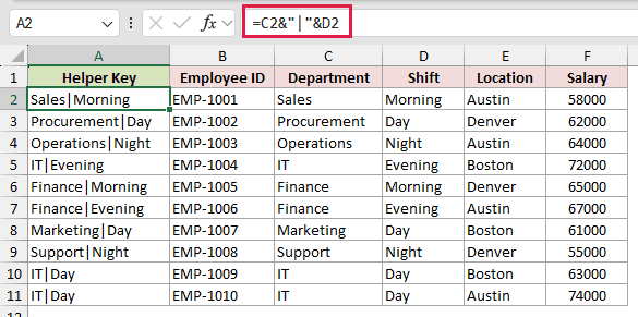
Now I’ll put the two criteria in their own cells, Finance in H2 and Evening in I2, and run a normal VLOOKUP against the helper column:

=VLOOKUP(H2&"|"&I2, A2:F11, 6, 0)

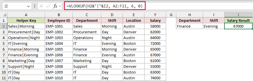
This returns 67000, the salary for the Finance Evening employee.

How does this formula work?

I build the same combined key from the criteria cells, H2&"|"&I2, which gives Finance|Evening. VLOOKUP searches the helper column for that exact key.

When it finds the match, it returns the value from the 6th column of the table A2:F11, which is Salary. The 0 forces an exact match, which is what you always want here.

Note: VLOOKUP can only return values that sit to the right of its lookup column. That’s why the helper column goes on the left. If you’d rather not move your columns around, Method #2 does the same job with VLOOKUP and leaves your data exactly as it is.

Method #2: Using VLOOKUP With the CHOOSE Function

Here’s another way to do this. If you’d rather not add a helper column to your sheet, you can build that combined column inside the formula itself.

This keeps your data untouched and does the whole lookup in one cell.

Here I’m back to the original roster with no helper column. The criteria go in two cells, Finance in G2 and Evening in H2.

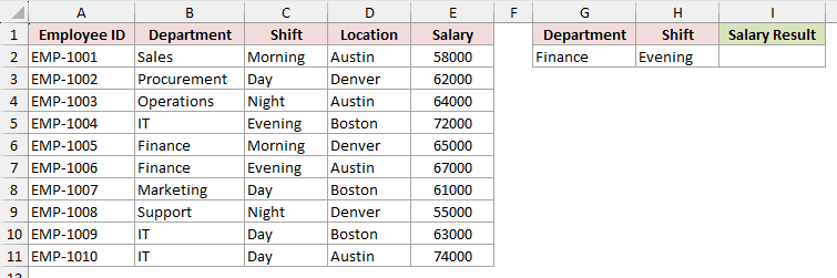
Here is the formula:

=VLOOKUP(G2&"|"&H2, CHOOSE({1,2}, B2:B11&"|"&C2:C11, E2:E11), 2, 0)

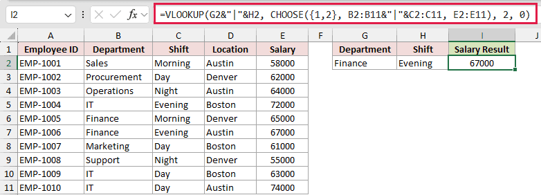
This returns 67000, the same salary as before.

How does this formula work?

The clever part is the CHOOSE call, CHOOSE({1,2}, B2:B11&"|"&C2:C11, E2:E11). It builds a two-column array in memory. The first column is Department joined to Shift, and the second is Salary.

VLOOKUP then treats that in-memory array as its table. It looks up Finance|Evening in the first column and returns the salary from the second.

Note: In Excel 2019 and earlier, this is an array formula. You must confirm it with Ctrl+Shift+Enter instead of just Enter, otherwise you’ll usually see a #VALUE! error. In Excel 2021 and later you can press Enter as usual.

Alternatives to VLOOKUP for Multiple Criteria

Methods #1 and #2 are the VLOOKUP answers. If VLOOKUP is what you’re stuck with, either because it’s already sitting in a file someone handed you or because your version of Excel doesn’t have the newer functions, those two are your options.

The four methods below solve the same problem, but none of them use VLOOKUP. Each one replaces it with a different function.

They’re shorter and easier to read, so they’re worth knowing if you’re free to choose. If you’re not, skip ahead to the three-criteria and different-sheet sections, which both cover the VLOOKUP way of doing it.

Method #3: Using the XLOOKUP Function

This method drops VLOOKUP and uses XLOOKUP instead. It needs Microsoft 365, Excel 2021, or Excel 2024, so skip it if you’re on an older version.

If you do have it, this is the method I’d actually use. XLOOKUP handles multiple criteria without a helper column and without the CHOOSE trick.

It also doesn’t care whether your answer sits left or right of the criteria.

I’m using the same roster, with Finance in G2 and Evening in H2.

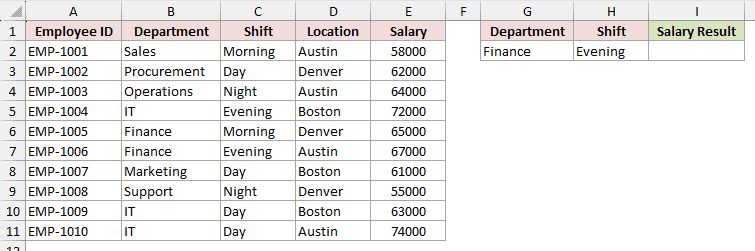
Here is the formula:

=XLOOKUP(G2&"|"&H2, B2:B11&"|"&C2:C11, E2:E11)

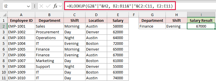
This returns 67000.

How does this formula work?

XLOOKUP takes the lookup value first, then the array to search, then the array to return from. There’s no column index to count, which is what makes it so much shorter than the VLOOKUP versions.

I join the criteria into Finance|Evening and search a matching joined array built from columns B and C. XLOOKUP finds it in row 6 of the range and returns the salary from the same position in column E.

There’s a second way to write it that skips the delimiter completely:

=XLOOKUP(1, (B2:B11=G2)*(C2:C11=H2), E2:E11)

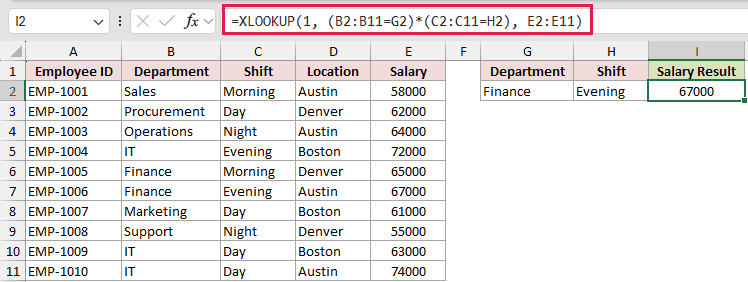
Each comparison gives an array of TRUE and FALSE values. Multiplying them turns those into 1s and 0s, and only the row where both conditions are true ends up as a 1.

XLOOKUP then looks for that 1. Since there’s no text being glued together, delimiter problems can’t happen at all.

Note: XLOOKUP takes an optional fourth argument for when nothing matches. =XLOOKUP(G2&”|”&H2, B2:B11&”|”&C2:C11, E2:E11, “Not found”) returns your own message instead of a #N/A error, which is much friendlier in a report someone else will read.

Method #4: Using INDEX and MATCH

This one drops VLOOKUP as well, but unlike XLOOKUP it works in every version of Excel. If you don’t have XLOOKUP, INDEX and MATCH gets you the same flexibility.

It handles multiple criteria without a helper column and doesn’t care which side of the sheet your answer sits on.

I’m using the same roster again, with Finance in G2 and Evening in H2.

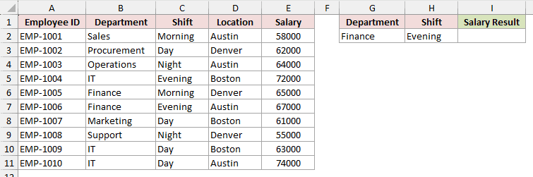
Here is the formula:

=INDEX(E2:E11, MATCH(G2&"|"&H2, B2:B11&"|"&C2:C11, 0))

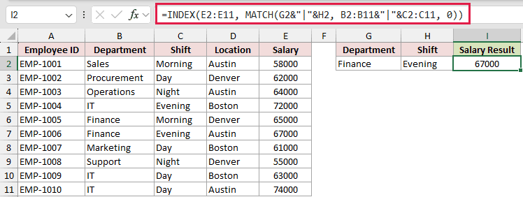
This returns 67000.

How does this formula work?

MATCH does the heavy lifting. It joins Department and Shift for every row, then finds the position of Finance|Evening in that list. Here that’s the 6th row of the range.

INDEX then grabs the 6th value from the Salary column E2:E11. The 0 in MATCH means exact match.

There’s more you can do with this pairing, including a non-array version for older Excel and the INDEX MATCH MATCH shape for grid-style data. I’ve covered all of it in INDEX MATCH with Multiple Criteria in Excel.

Note: Just like Method #2, the concatenated MATCH is an array formula in Excel 2019 and earlier, so confirm it with Ctrl+Shift+Enter. In Excel 2021 and later a plain Enter works fine.

Method #5: Using the FILTER Function to Return Every Match

FILTER isn’t a lookup function and has nothing to do with VLOOKUP. It also needs Microsoft 365, Excel 2021, or Excel 2024.

It earns its place because every method so far returns one answer. FILTER returns all of them, which matters when your criteria match more than one row.

It’s the only method here that gives you the full list rather than just the first hit.

This time I’m looking for everyone in the IT department on the Day shift, with IT in G2 and Day in H2. Two people in the roster fit.

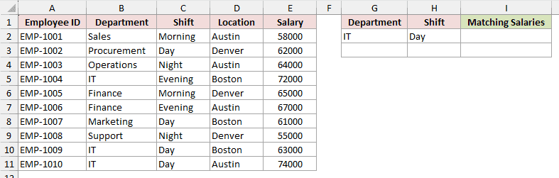
Here is the formula:

=FILTER(E2:E11, (B2:B11=G2)*(C2:C11=H2))

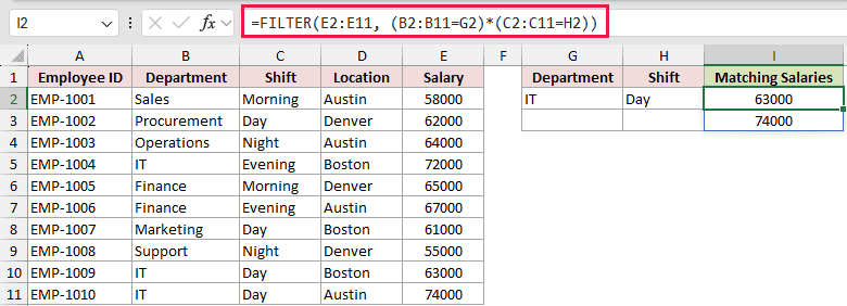
The formula spills down the column automatically and returns both salaries, 63000 and 74000.

How does this formula work?

The first argument is what I want back, the Salary column. The second is the condition, and it’s the same multiplication trick from Method #3.

(B2:B11=G2)*(C2:C11=H2) gives a 1 for every row where the department is IT and the shift is Day, and a 0 everywhere else. FILTER keeps the rows that scored a 1 and drops the rest.

Because two rows qualify, you get two results. Methods #1 to #4 would have quietly handed you 63000 and left you thinking that was the only answer, and SUMIFS would have added the two together into 137000.

Note: FILTER needs Microsoft 365, Excel 2021, or Excel 2024. Make sure the cells below the formula are empty, or you’ll get a #SPILL! error. To handle no matches at all, add a third argument: =FILTER(E2:E11, (B2:B11=G2)*(C2:C11=H2), “No match”).

Method #6: Using SUMIFS When the Result Is a Number

If the value you’re pulling back is a number, you don’t need a lookup function at all. This method replaces VLOOKUP with a math function, and it works in every version of Excel.

SUMIFS was built to handle multiple criteria. It takes them as plain arguments, so there’s no array to build and no Ctrl+Shift+Enter in any version of Excel.

I’m back to Finance in G2 and Evening in H2, pulling the salary.

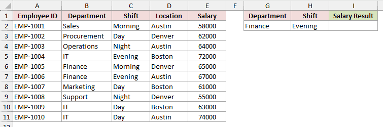
Here is the formula:

=SUMIFS(E2:E11, B2:B11, G2, C2:C11, H2)

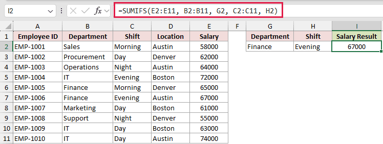
This returns 67000, the same answer every other method gave.

How does this formula work?

The first argument is the column to add up, Salary. After that come the criteria in pairs: the range to check, then what to check it against.

So it adds up every salary where the department is Finance and the shift is Evening. Only one row qualifies, so the “sum” is just that one salary.

Note: This only works when the result is numeric, and it adds instead of looking up. If two rows match, you get their total rather than the first value, and if nothing matches you get 0 rather than #N/A. That makes it a great sanity check but a poor fit for text results.

How to Look Up With Three or More Criteria in Excel

Two criteria aren’t always enough. In my roster, IT plus Day matches two different people, so those two conditions can’t tell them apart.

Adding the Location column as a third criterion fixes that. Here I want IT, Day, and Austin, sitting in G2, H2, and I2.

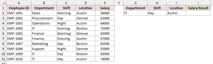
Here is the formula:

=XLOOKUP(1, (B2:B11=G2)*(C2:C11=H2)*(D2:D11=I2), E2:E11)

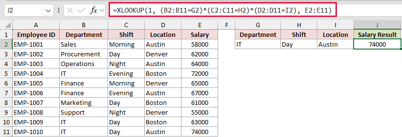
This returns 74000, the Austin employee, not the 63000 one in Boston.

The multiplication approach scales to as many criteria as you need. Just multiply in another bracket for each one, and a row has to satisfy every condition to come back as a 1.

The same idea works with the concatenation style too. Join all three criteria with your delimiter on both sides of the formula, and INDEX MATCH takes extra criteria the same way.

If you need to do this with VLOOKUP, both VLOOKUP methods stretch to three criteria without any trouble. The CHOOSE version from Method #2 just gets a third piece joined into the key on each side:

=VLOOKUP(G2&"|"&H2&"|"&I2, CHOOSE({1,2}, B2:B11&"|"&C2:C11&"|"&D2:D11, E2:E11), 2, 0)

That returns the same 74000. It’s an array formula in Excel 2019 and earlier, so confirm it with Ctrl+Shift+Enter there, just like Method #2.

The helper column from Method #1 works the same way. Join the third column into the helper formula, then look up all three criteria joined in the same order.

How to Use VLOOKUP With Criteria on a Different Sheet

Your lookup table often lives on its own sheet. The logic doesn’t change at all. You just point the ranges at the other sheet.

Here my roster sits on a sheet called Employee Data.

On a second sheet called Lookup, I’ve put Finance in A2 and Evening in B2, and the result goes in C2.

Here’s the VLOOKUP version, using the CHOOSE approach from Method #2:

=VLOOKUP(A2&"|"&B2, CHOOSE({1,2}, 'Employee Data'!B2:B11&"|"&'Employee Data'!C2:C11, 'Employee Data'!E2:E11), 2, 0)

This returns 67000, exactly as it did when everything was on one sheet. In Excel 2019 and earlier, confirm it with Ctrl+Shift+Enter.

The helper column from Method #1 crosses sheets just as happily. Build the helper column on the data sheet, then point VLOOKUP’s second argument at it, as in 'Employee Data'!A2:F11.

And here’s the same lookup with XLOOKUP, if you have it:

=XLOOKUP(A2&"|"&B2, 'Employee Data'!B2:B11&"|"&'Employee Data'!C2:C11, 'Employee Data'!E2:E11)

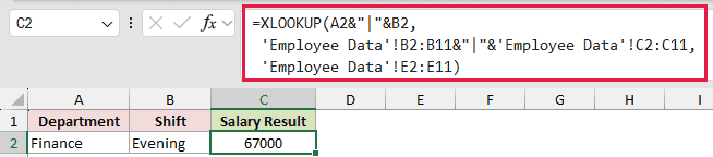
That returns 67000 too, in a much shorter formula.

The sheet name goes in front of each range with an exclamation mark. Excel adds the single quotes automatically when the name has a space in it, as Employee Data does.

The easiest way to get this right is to start typing the formula, then click across to the other sheet and drag over the range. Excel writes the reference for you.

Additional Notes About Using VLOOKUP with Multiple Criteria in Excel

• Always use a delimiter like | when you join criteria. Without one, a 12 joined to a 3 and a 1 joined to a 23 both come out as 123, and you can get a wrong match. Pick a character that never appears in your actual data.
• These lookups are not case sensitive, so finance and Finance are treated as the same value. Trim stray spaces too, since a trailing space makes an otherwise identical key fail to match.
• If more than one row shares the same criteria combination, Methods #1 to #4 return the first match only, and SUMIFS adds every match together. Add another criterion, or switch to FILTER, when duplicates are possible.
• VLOOKUP returns a #VALUE! error when its lookup value is longer than 255 characters, which combined keys can reach on wide real-world data. MATCH has the same limit, so Method #4 doesn’t rescue you. XLOOKUP and the multiplication forms take a key of any length.
• The multiplication approach needs the ranges to be the same size. Mixing B2:B11 with C2:C12 gives a #VALUE! error.

Frequently Asked Questions

Can VLOOKUP match on two columns at once natively?

No. VLOOKUP only accepts a single lookup value and searches a single column. To match on two conditions you either combine the criteria into one value or switch to a function like XLOOKUP, INDEX MATCH, or FILTER.

Which of these methods actually use VLOOKUP?

Only the first two. Method #1 (helper column) and Method #2 (CHOOSE) are VLOOKUP formulas, and both also cover the three-criteria and different-sheet cases further down. Methods #3 to #6 replace VLOOKUP with XLOOKUP, INDEX MATCH, FILTER, and SUMIFS, so they only help if you’re free to move off VLOOKUP.

Why does my VLOOKUP with multiple criteria return #N/A?

Usually the combined key doesn’t match exactly. Common causes are a different delimiter or column order between the two keys, extra spaces in the data, or forgetting Ctrl+Shift+Enter in older Excel. VLOOKUP Not Working walks through the rest.

How do I look up with three criteria in Excel?

Multiply a third condition into the formula, as in =XLOOKUP(1, (B2:B11=G2)*(C2:C11=H2)*(D2:D11=I2), E2:E11). The same pattern extends to four or more criteria.

Can I get all the matching rows instead of just the first?

Yes, that’s what Method #5 is for. FILTER returns every row that satisfies your criteria and spills them down the sheet. The other methods stop at the first hit.

Is XLOOKUP better than VLOOKUP for multiple criteria?

For most people, yes. XLOOKUP is shorter, doesn’t need a helper column or CHOOSE, and handles missing values with its own argument. It just isn’t available in Excel 2019 or earlier, which is where the VLOOKUP methods still earn their keep.

Conclusion

Multiple-criteria lookups come down to giving Excel one combined value to match on, or one array of 1s and 0s to search.

If it has to be VLOOKUP, you have two choices. The helper column is the easiest to set up and troubleshoot, and it’s what I’d pick if someone else has to maintain the file. The CHOOSE version does the same job in one cell when you can’t add a column.

If you’re free to use something else, and you have Microsoft 365, Excel 2021, or Excel 2024, use XLOOKUP and stop there. On an older version without XLOOKUP, INDEX MATCH is the one to reach for.

And when your criteria might match several rows, reach for FILTER so you see all of them rather than just the first.

Other Excel articles you may also like:

• XLOOKUP Vs INDEX MATCH in Excel
• How to Use Wildcard in XLOOKUP
• Using VLOOKUP Approximate Match in Excel (Examples)
• VLOOKUP in Power Query
• How to Compare Two Columns in Excel (using VLOOKUP & IF)