
If you want to know exactly how many characters sit inside a cell, Excel can tell you in a second, no manual counting required.
The tricky part is that “characters” can mean the full total, one specific letter, or the count with spaces stripped out. Each of those needs a slightly different formula.
Good news: they’re all short, and once you’ve seen them you’ll reuse them everywhere. Below I’ll walk through four ways to count characters in a cell, from a plain total to counting a single character across a whole column.
Method #1: Using the LEN Function
The LEN function is the one you’ll reach for most. Hand it a cell and it returns the number of characters in that cell, counting letters, numbers, spaces, and punctuation alike.
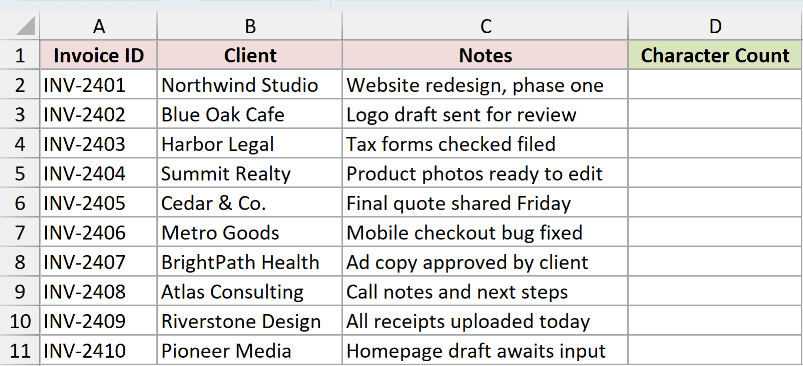
Below I have a list of freelance invoices. Each row has an Invoice ID, the client name, and a short Notes field. I want to count the characters in each note.
Here is the formula:
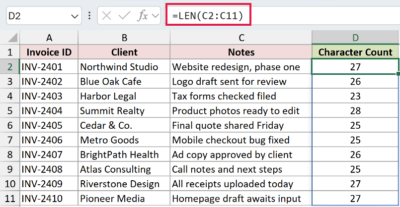
=LEN(C2:C11)
Enter it once in D2 and it spills down the column automatically, giving you a count for every note.
How does this formula work?
LEN reads whatever text is in the cell and returns its length. For the note in C2, “Website redesign, phase one”, it returns 27. That total includes the three spaces and the comma, not just the letters.
Because I passed the whole range C2:C11 in one go, the single formula spills a result next to each row. In older versions without dynamic arrays, put =LEN(C2) in D2 and fill it down instead.
Note: LEN counts every character, including leading and trailing spaces. If a cell looks shorter than its count suggests, use =LEN(TRIM(C2)) to remove leading and trailing spaces and reduce repeated spaces between words to one before counting.
Method #2: Using LEN and SUBSTITUTE (One Specific Character)
Sometimes you don’t want the full total, you want to know how many times one specific character shows up. There’s no single function for that, but a neat LEN and SUBSTITUTE combo does the job.
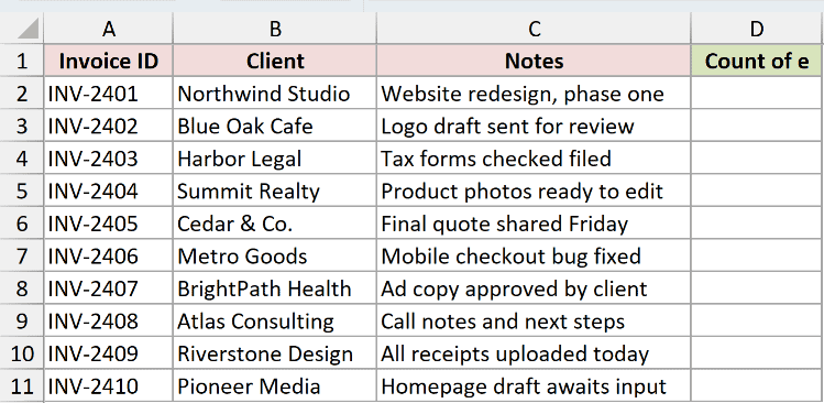
I’m using the same invoice list, and this time I want to count how many times the letter “e” appears in each note.
The idea is simple. First, strip out every “e” using SUBSTITUTE, then compare the shortened length to the original. Here is what SUBSTITUTE returns on its own for the first note:
=SUBSTITUTE(C2,"e","")
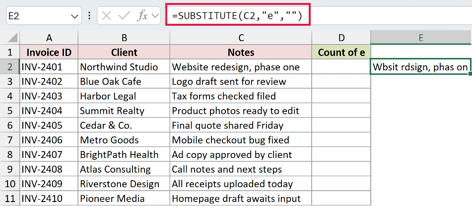
That turns “Website redesign, phase one” into “Wbsit rdsign, phas on”. Now wrap the whole thing in the counting formula:
=LEN(C2:C11)-LEN(SUBSTITUTE(C2:C11,"e",""))
In Excel 365 or Excel 2021, this formula spills down automatically. In Excel 2019 or earlier, use =LEN(C2)-LEN(SUBSTITUTE(C2,”e”,””)) and copy it down.
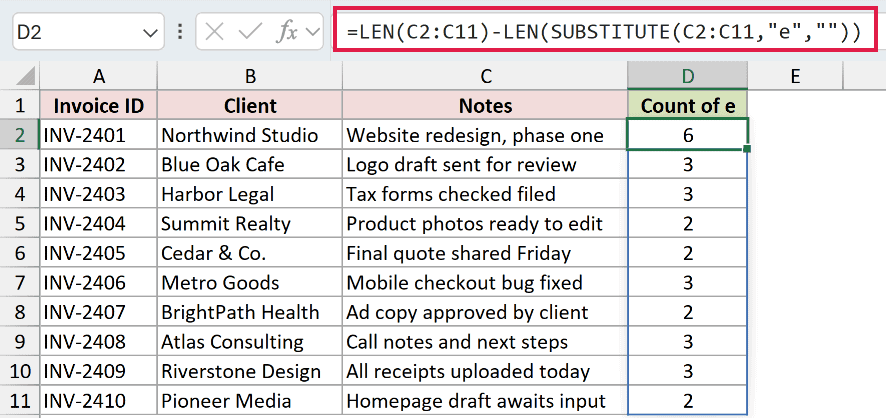
How does this formula work?
LEN(C2:C11) gives the original length of each note. SUBSTITUTE(C2:C11,"e","") removes every “e”, and wrapping that in LEN gives the shorter length. Subtract the two and you’re left with how many “e” characters were removed.
For C2 the original length is 27 and the stripped length is 21, so the formula returns 6. Change the “e” to any letter, digit, or symbol to count that character instead.
Note: SUBSTITUTE is case sensitive, so “e” and “E” are counted separately. To count both regardless of case, run the text through UPPER or LOWER first, like =LEN(C2)-LEN(SUBSTITUTE(LOWER(C2),”e”,””)).
Method #3: Using SUMPRODUCT and LEN (Whole Column Total)
The first method counts each cell on its own. When you want one grand total, the number of characters across an entire column, SUMPRODUCT adds up the individual LEN results for you in a single cell.
Here’s the same invoice notes column. This time I want one number: the total characters across all ten notes.
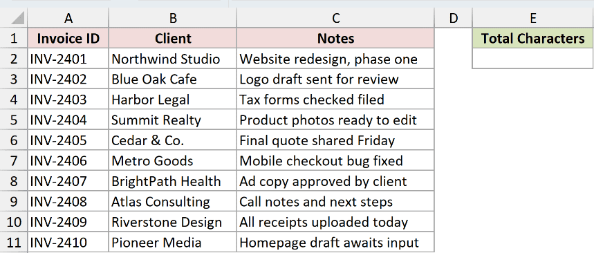
Here is the formula:
=SUMPRODUCT(LEN(C2:C11))
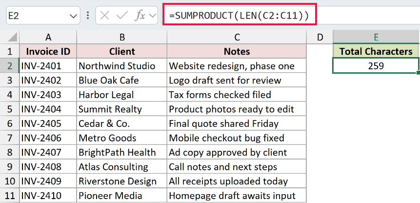
How does this formula work?
LEN(C2:C11) hands SUMPRODUCT an array of ten lengths, one per note. SUMPRODUCT then adds that array into a single value, so I don’t have to sum a helper column myself.
For my data the total comes to 259. =SUM(LEN(C2:C11)) returns the same total in Excel 365 or Excel 2021, but SUMPRODUCT works even in older versions without you pressing Ctrl+Shift+Enter.
Method #4: Using LEN and SUBSTITUTE (Excluding Spaces)
Spaces count as characters, which throws people off when they only care about the visible text. To count characters while ignoring spaces, strip the spaces out with SUBSTITUTE first, then measure the length.
I’ll use the invoice notes again and count each note’s characters with the spaces removed.
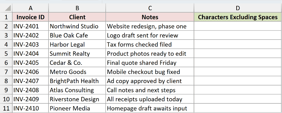
Here is the formula:
=LEN(SUBSTITUTE(C2:C11," ",""))
In Excel 365 or Excel 2021, this formula spills down automatically. In Excel 2019 or earlier, use =LEN(SUBSTITUTE(C2,” “,””)) and copy it down.
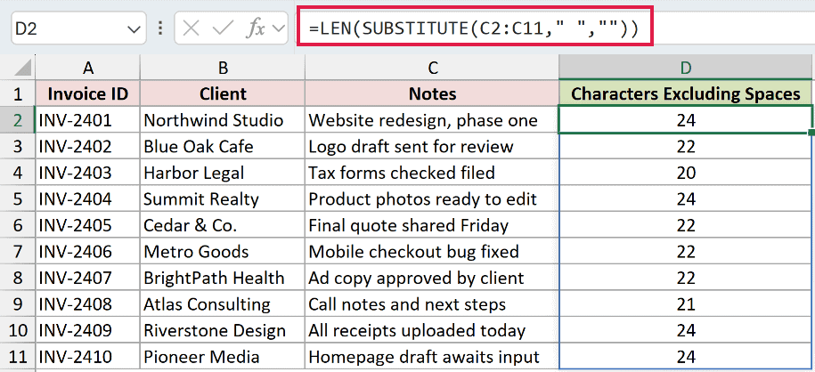
How does this formula work?
SUBSTITUTE(C2:C11," ","") replaces every space with nothing, so the note becomes one unbroken string. Wrapping that in LEN then measures the length of that space-free text.
The note in C2 has 27 characters and three spaces, so the formula returns 24. This only removes the standard space character, so line breaks or non-breaking spaces would still be counted.
Note: To count characters excluding all spaces across the whole column at once, wrap this in SUMPRODUCT: =SUMPRODUCT(LEN(SUBSTITUTE(C2:C11,” “,””))).
Additional Notes About Counting Characters in Excel
- A single Excel cell holds up to 32,767 characters, so LEN will never return a number higher than that for one cell.
- LEN counts invisible characters too. Trailing spaces, tabs, and line breaks all add to the total, which is why a count can look larger than expected.
- LENB is deprecated in current Excel. It remains for compatibility with older workbooks that count bytes in double-byte character set languages, but use LEN for new character-count formulas.
- LEN treats numbers as text for counting, so
=LEN(1234)returns 4. Formatting like currency symbols or commas is not part of the stored value and is not counted.
Frequently Asked Questions
Is there a character limit for text in a single Excel cell?
Yes. A cell can store up to 32,767 characters. Even when the cell doesn’t display all of it, the text is still there and still counted by LEN.
Why does my character count include spaces I did not add?
Extra spaces often hide at the start or end of a cell, or double up between words. Wrap the reference in TRIM, like =LEN(TRIM(C2)), to drop leading, trailing, and repeated spaces before counting.
How do I count one specific character across an entire column at once?
Combine the Method #2 trick with SUMPRODUCT: =SUMPRODUCT(LEN(C2:C11)-LEN(SUBSTITUTE(C2:C11,"e",""))). This adds up every “e” in the whole range and returns a single total, which is 29 for my invoice notes.
Conclusion
Counting characters in Excel comes down to LEN and a couple of helpers.
Reach for =LEN() for a plain per-cell total, pair it with SUBSTITUTE when you need a specific character or want to skip spaces, and wrap either in SUMPRODUCT to total a whole column. For most jobs, plain LEN is all you’ll need.
Other Excel articles you may also like:
