
If you want to find the first, second, third, or any other ranked value in a list, the LARGE function is what you need.
LARGE returns one value when you give it one rank. It also works inside dynamic array formulas, where functions such as SEQUENCE can supply several ranks at once.
In this article, I’ll show you how to find ranked values, build a top-values list, add the top results, apply conditions, ignore duplicates, and return a matching label.
LARGE Function Syntax in Excel
The LARGE function uses the following syntax:
=LARGE(array, k)
arrayis the required array or cell range that contains the numbers.kis the required position counted from the largest value. Use 1 for the largest, 2 for the second largest, and so on.
If you need only the single highest number, our guide to finding the largest value in Excel also covers MAX and other approaches.
When to Use LARGE Function
- Return the nth-largest number from a list.
- Create a ranked list of the top few values.
- Add the largest values without sorting the source data.
- Find a ranked value after filtering the list by a condition.
- Return a label associated with a ranked number.
Example 1: Find the Third-Highest Repair Estimate
Start with a simple ranking.
Below is a list of facilities and their repair estimates.
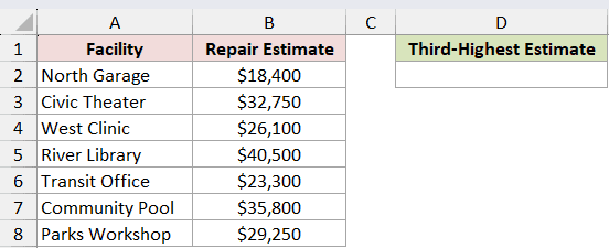
I want to return the third-highest estimate without sorting the facility list.
Here is the formula:
=LARGE(B2:B8,3)
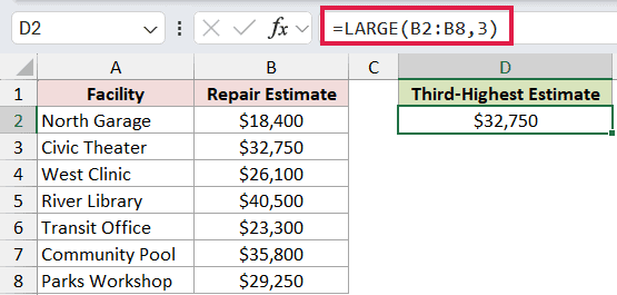
The array is B2:B8, and k is 3. Excel ranks the estimates from largest to smallest and returns $32,750, the third-highest amount.
The source list stays in its original order. LARGE performs the ranking inside the formula.
Example 2: Return Several Top Values by Rank
You can keep the rank in a worksheet cell instead of typing it directly into the formula.
Below is a parcel-count dataset with positions 1 through 4 in D2:D5.
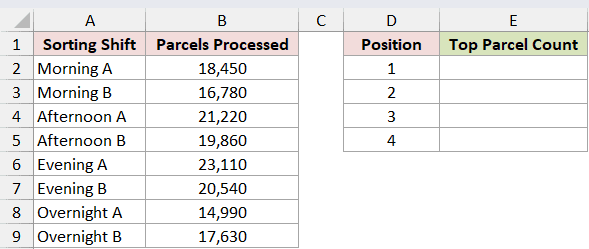
I want to return the parcel count for each listed position.
Enter this formula in E2 and copy it down to E5:
=LARGE($B$2:$B$9,D2)
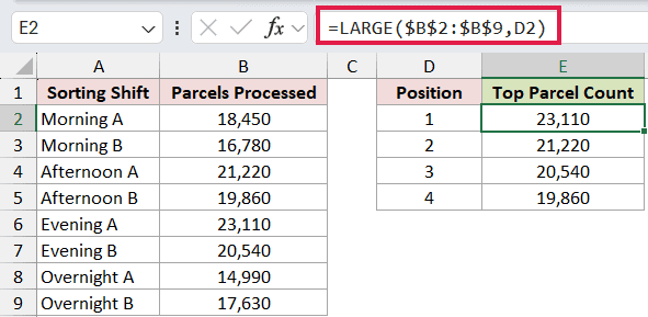
The absolute reference keeps B2:B9 fixed while D2 changes as the formula moves down. The results are 23,110, 21,220, 20,540, and 19,860.
In Excel 365 or Excel 2024, =TAKE(SORT(B2:B9,1,-1),4) is a cleaner option when you want the complete top-four list to spill from one formula. LARGE remains useful when the ranks come from worksheet cells.
Example 3: Sum the Top Three Visitor Counts
LARGE can return several ranked values inside another formula.
Below is a list of galleries and their weekend visitor counts.
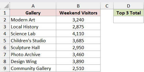
I want to add the three highest visitor counts.
Here is the formula:
=SUM(LARGE(B2:B9,SEQUENCE(3)))
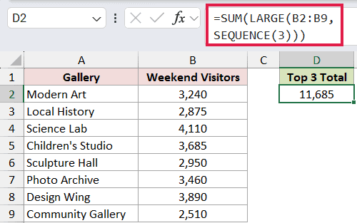
The SEQUENCE function supplies the ranks 1, 2, and 3. LARGE returns 4,110, 3,890, and 3,685, then SUM combines them to give 11,685.
This formula needs a version of Excel that supports SEQUENCE. In older versions, list the ranks in cells and use the approach from Example 2.
Example 4: Find an Nth-Largest Value by Queue
You can filter the numbers before LARGE ranks them.
Below is a support-ticket list with queue names and resolution hours. The selected queue is Billing, and the requested rank is 2.
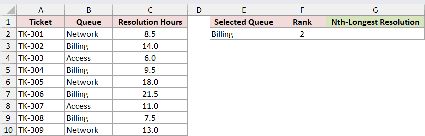
I want to return the second-longest resolution time for Billing tickets only.
Here is the formula:
=LARGE(FILTER(C2:C10,B2:B10=E2),F2)
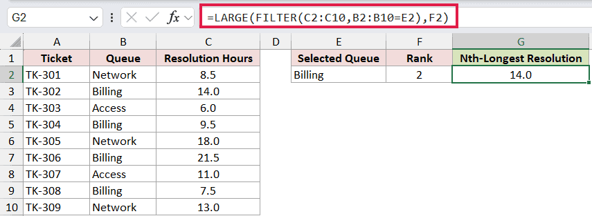
The FILTER function keeps the four Billing times: 14, 9.5, 21.5, and 7.5 hours. LARGE then returns 14, the second-highest value in that filtered array.
FILTER is available in Microsoft 365, Excel 2024, and Excel 2021. In older Excel versions, use a helper column or an array formula designed for that version.
Pro Tip: If no rows match the selected queue, FILTER returns #CALC! before LARGE can rank anything. Validate the queue name, or wrap the complete formula in IFERROR when you want a friendly message.
Example 5: Find the Second-Highest Distinct Quote
Duplicate numbers take separate positions in a normal LARGE calculation.
Below is a freight-quote list where several carriers submitted the same amount.
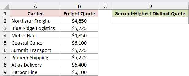
I want the second-highest distinct quote, so repeated amounts should count only once.
Here is the formula:
=LARGE(UNIQUE(B2:B9),2)
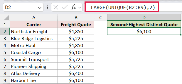
The UNIQUE function removes repeated quotes before LARGE ranks them. The distinct values put $6,400 first and $6,100 second, so the formula returns $6,100.
Without UNIQUE, both $6,100 quotes would occupy separate ranks. This formula requires Microsoft 365, Excel 2024, or Excel 2021.
Example 6: Return the Value and Project at a Rank
Here is a practical way to pair a ranked amount with its project.
Below is a project list with estimated annual savings and a requested rank of 2.
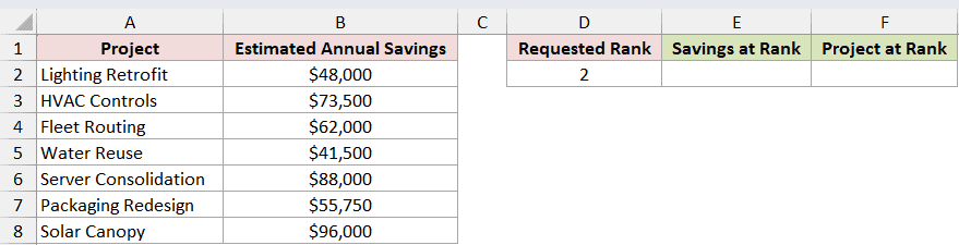
I want to return both the savings amount and the project in second place.
Here is the formula for the savings amount:
=LARGE(B2:B8,D2)
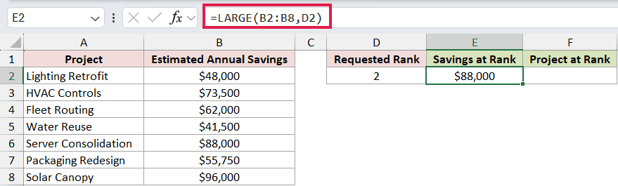
LARGE returns $88,000, the second-highest estimated saving.
Then use that amount as the lookup value:
=XLOOKUP(LARGE(B2:B8,D2),B2:B8,A2:A8)
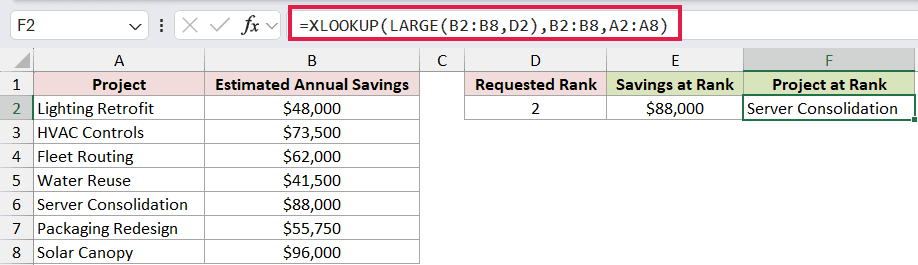
The XLOOKUP function finds $88,000 in column B and returns Server Consolidation from column A.
If two projects have the same savings value, XLOOKUP returns the first match. Use FILTER instead when you need every project tied at that rank.
Tips & Common Mistakes
kmust be greater than zero and cannot exceed the number of numeric data points. Otherwise, LARGE returns#NUM!.- LARGE also returns
#NUM!when the supplied array is empty. - Duplicate values occupy separate ranks unless you remove them first with UNIQUE.
- LARGE returns one value for a single
k. When a dynamic array supplies several ranks, LARGE can return several values for another function to use or for Excel to spill. - You can use a spilled range as the array, such as
=LARGE(B2#,3), when the source list already comes from a dynamic array formula. - A blocked spill area returns
#SPILL!. Implicit intersection reduces an array result to one value. - LARGE is available in Excel 2016 and later. SEQUENCE, FILTER, UNIQUE, and XLOOKUP require newer versions that include those functions.
I’ve shown you how to use LARGE for single ranks, top-value lists, filtered rankings, distinct values, totals, and matching labels. I hope you found this article helpful.
Related Excel Functions / Articles:
Other Excel articles you may also like:
