
Excel’s F.DIST.RT function returns the probability of an F value exceeding a specified statistic. This is the area in the distribution’s right tail.
For an appropriate F-test, that probability is a p-value. A small result means the observed statistic would be unusual under the null hypothesis.
F.DIST.RT Function Syntax in Excel
F.DIST.RT takes three required arguments:
=F.DIST.RT(x,deg_freedom1,deg_freedom2)
- x: The F statistic to evaluate. It must be zero or greater.
- deg_freedom1: The numerator degrees of freedom, at least 1.
- deg_freedom2: The denominator degrees of freedom, at least 1.
When to Use F.DIST.RT Function
- Convert a table of F statistics and degrees of freedom into right-tail p-values.
- Test whether one population variance is greater than another using sample data.
- Work through a two-tailed variance comparison and check it with F.TEST.
- Calculate the p-value for a one-way ANOVA.
- Calculate the overall regression p-value, also called Significance F.
Example 1: Calculate p-Values for Multiple F Statistics
Let’s start with a list of completed menu tests.
Below is the dataset showing six menu tests, their F statistics, both degrees of freedom, and Alpha in I2. The labelled p-Value and Decision cells are empty.
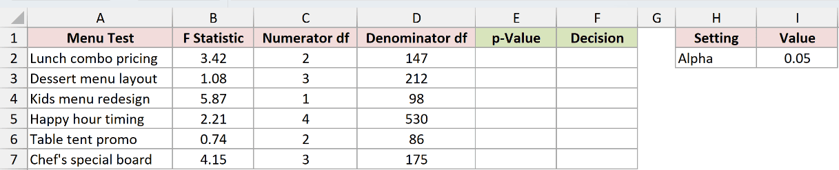
We want one p-value per test, followed by a decision using the 0.05 threshold in I2.
Enter the formula in E2.
Here is the formula:
=F.DIST.RT(B2:B7,C2:C7,D2:D7)
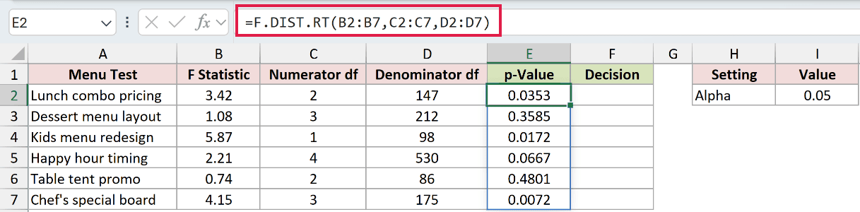
The formula matches each F statistic in B2:B7 with the corresponding degrees of freedom in C2:C7 and D2:D7.
In Excel 2021, Excel 2024 and Microsoft 365, the six results spill into E2:E7 automatically.
Lunch combo pricing returns 0.0353, while Dessert menu layout returns 0.3585. These are displayed values rounded to four decimal places.
To label each result, enter this formula in F2:
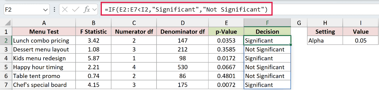
=IF(E2:E7<I2,"Significant","Not Significant")
How this formula works:
E2:E7<I2compares each unrounded p-value with Alpha, 0.05.- IF returns “Significant” when the comparison is TRUE and “Not Significant” otherwise.
- The decisions spill into F2:F7. Lunch combo pricing, Kids menu redesign, and Chef’s special board return “Significant”.
Pro Tip: These are separate comparisons against 0.05, without an adjustment for multiple testing. In Excel 2019 and earlier, calculate each row separately and fill down, keeping the Alpha reference fixed.
Example 2: Test Whether One Variance Is Greater
Now let’s calculate the F statistic from delivery times.
Below is the dataset with 10 current-courier delivery times in A2:A11 and 12 new-courier times in B2:B13. The Metric labels have empty Result cells beside them.
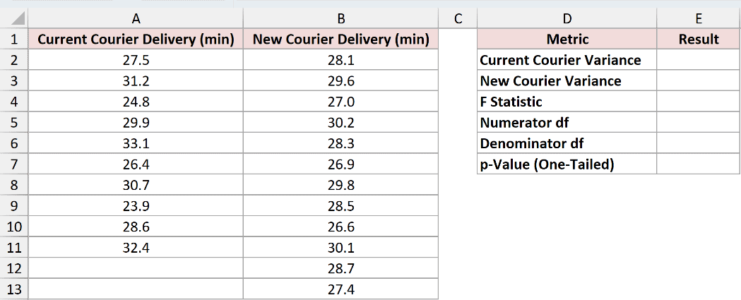
We want to test whether the current courier has greater delivery-time variance than the new courier.
How the card is built:
- E2:
=VAR.S(A2:A11)uses VAR.S to calculate the current courier’s sample variance, displayed as 9.945. - E3:
=VAR.S(B2:B13)returns the new courier’s sample variance, displayed as 1.652. Both variances are in squared minutes. - E4:
=E2/E3returns 6.022. The current courier goes in the numerator because we’re testing whether its population variance is greater. - E5:
=COUNT(A2:A11)-1returns 9 numerator degrees of freedom from 10 current-courier observations. - E6:
=COUNT(B2:B13)-1returns 11 denominator degrees of freedom from 12 new-courier observations.
Finally, enter the right-tail probability formula in E7:
=F.DIST.RT(E4,E5,E6)
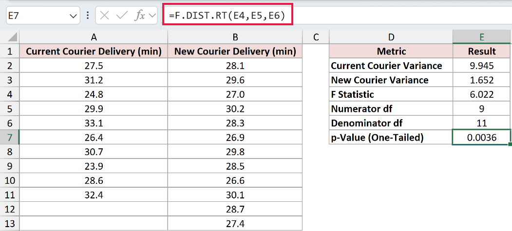
F.DIST.RT uses the F statistic in E4 and degrees of freedom 9 and 11. The p-value displays as 0.0036.
At a 0.05 significance level, this supports greater population variance for the current courier, assuming the variance-test conditions hold.
Pro Tip: Choose the direction before examining the results. This classical variance test assumes independent observations from normally distributed populations. F.TEST returns a two-tailed p-value, so it answers a different question.
Example 3: Compare Variances with a Two-Tailed Test
A question about any difference needs a two-tailed calculation.
Below is the dataset with 12 day-shift pick times in A2:A13 and 10 night-shift times in B2:B11. The labelled calculation cells in E2:E9 are empty.
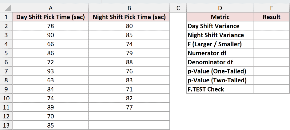
We want to test whether day-shift and night-shift population variances differ, regardless of direction.
How the card is built:
- E2:
=VAR.S(A2:A13)returns the day-shift sample variance, displayed as 100.697. - E3:
=VAR.S(B2:B11)returns the night-shift sample variance, displayed as 26.944. The day shift has the larger variance here. - E4:
=MAX(E2,E3)/MIN(E2,E3)divides the larger variance by the smaller one, returning 3.737. The day shift is the numerator for these data. - E5:
=COUNT(A2:A13)-1returns 11 numerator degrees of freedom from 12 day-shift observations. - E6:
=COUNT(B2:B11)-1returns 9 denominator degrees of freedom from 10 night-shift observations.
In E7, calculate the right-tail probability first:
=F.DIST.RT(E4,E5,E6)
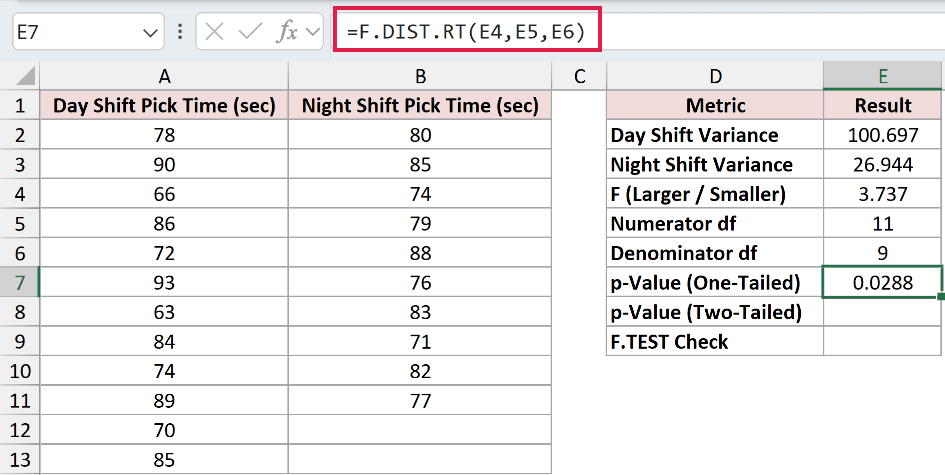
The result displays as 0.0288. This is the one-tailed probability for the supplied F statistic and degrees of freedom.
In E8, calculate the two-tailed p-value for these data:
=2*F.DIST.RT(E4,E5,E6)
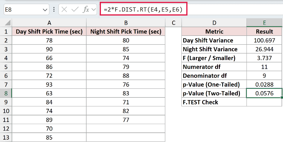
Doubling this right-tail probability returns 0.0576. At a 0.05 significance level, we do not reject equal population variances.
Using 0.0288 would suggest a significant difference at 0.05. Our two-tailed question needs 0.0576, which is above that threshold.
In E9, check the result directly from the samples:
=F.TEST(A2:A13,B2:B11)
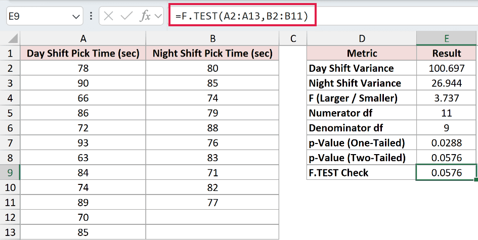
F.TEST also returns 0.0576. It is the shorter option when you need the two-tailed result directly from two sample ranges.
Pro Tip: Doubling matches F.TEST here, not universally. If the larger-variance sample changes, swap its degrees of freedom too. The references in E5:E6 stay fixed.
Example 4: Calculate an ANOVA p-Value
Let’s compare mean sales across three shelf placements.
Below is the dataset with six observations each for Endcap Units, Eye Level Units, and Bottom Shelf Units in A2:C7. The ANOVA metric labels have empty results.
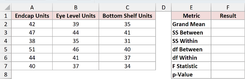
We want to test whether all three population means are equal using a one-way ANOVA.
How the card is built:
- F2:
=AVERAGE(A2:C7)calculates the grand mean across all 18 observations, displayed as 40.11 units. - F3:
=COUNT(A2:A7)*(AVERAGE(A2:A7)-F2)^2+COUNT(B2:B7)*(AVERAGE(B2:B7)-F2)^2+COUNT(C2:C7)*(AVERAGE(C2:C7)-F2)^2returns 161.78. It weights each squared difference between a group mean and the grand mean by that group’s observation count. - F4:
=DEVSQ(A2:A7)+DEVSQ(B2:B7)+DEVSQ(C2:C7)adds squared deviations from each group’s own mean, returning 272.00. - F5:
=COLUMNS(A2:C7)-1returns 2 between-group degrees of freedom from three groups. - F6:
=COUNT(A2:C7)-COLUMNS(A2:C7)subtracts three groups from 18 observations, returning 15 within-group degrees of freedom.
In F7, calculate the ANOVA F statistic:
=(F3/F5)/(F4/F6)
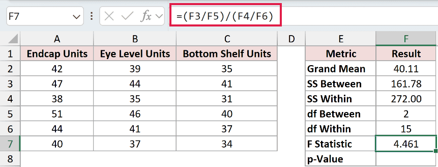
How this formula works:
F3/F5divides the between-group sum of squares by its degrees of freedom.F4/F6does the same for the within-group sum of squares.- Dividing these mean squares returns an F statistic displayed as 4.461.
In F8, calculate the right-tail p-value:
=F.DIST.RT(F7,F5,F6)
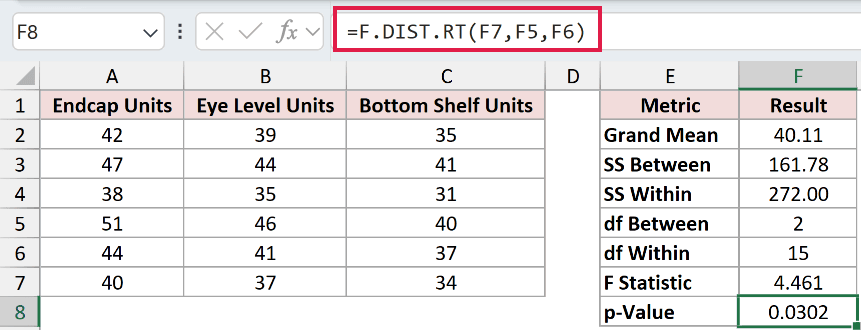
Using degrees of freedom 2 and 15, F.DIST.RT returns 0.0302. At a 0.05 significance level, we reject the hypothesis that all three means are equal.
This is the p-value calculated for the same data by the Data Analysis ToolPak’s Anova: Single Factor procedure.
Pro Tip: A significant ANOVA result needs follow-up comparisons to identify which pairs of means differ. This model assumes independent observations, normally distributed errors within groups, and equal population variances.
Example 5: Calculate Regression Significance F
We can also use F.DIST.RT to evaluate a regression model overall.
Below is the dataset showing Month, Social Ad Spend, Flyers Handed Out, and New Members for January through December. The regression metrics in F2:F5 have empty results.
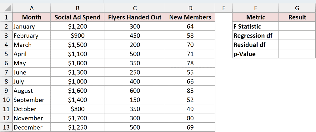
We want the overall regression p-value for predicting New Members from Social Ad Spend and Flyers Handed Out.
How the card is built:
- G3:
=COLUMNS(B2:C13)counts two predictor columns, giving 2 numerator degrees of freedom. - G4:
=INDEX(LINEST(D2:D13,B2:C13,TRUE,TRUE),4,2)returns 9 residual degrees of freedom: 12 observations minus two predictors and an intercept.
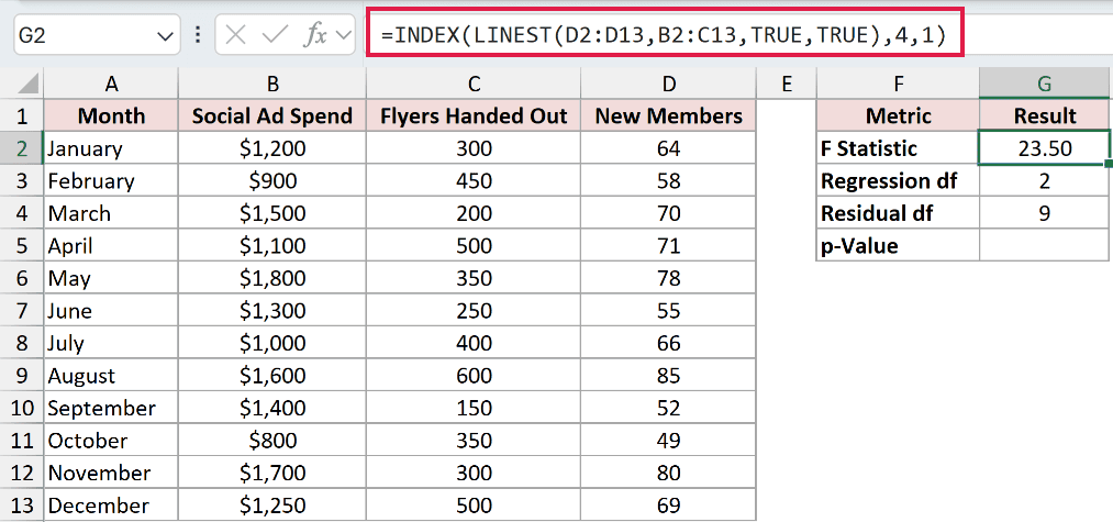
Enter the formula in G2 to extract the regression F statistic.
Here is the formula:
=INDEX(LINEST(D2:D13,B2:C13,TRUE,TRUE),4,1)
How this formula works:
- LINEST uses D2:D13 as the outcome and B2:C13 as the two predictor columns.
- The first TRUE includes an intercept. The second TRUE requests additional regression statistics.
- INDEX selects row 4, column 1 of those statistics. The F statistic displays as 23.50.
In G5, calculate the overall regression p-value:
=F.DIST.RT(G2,G3,G4)
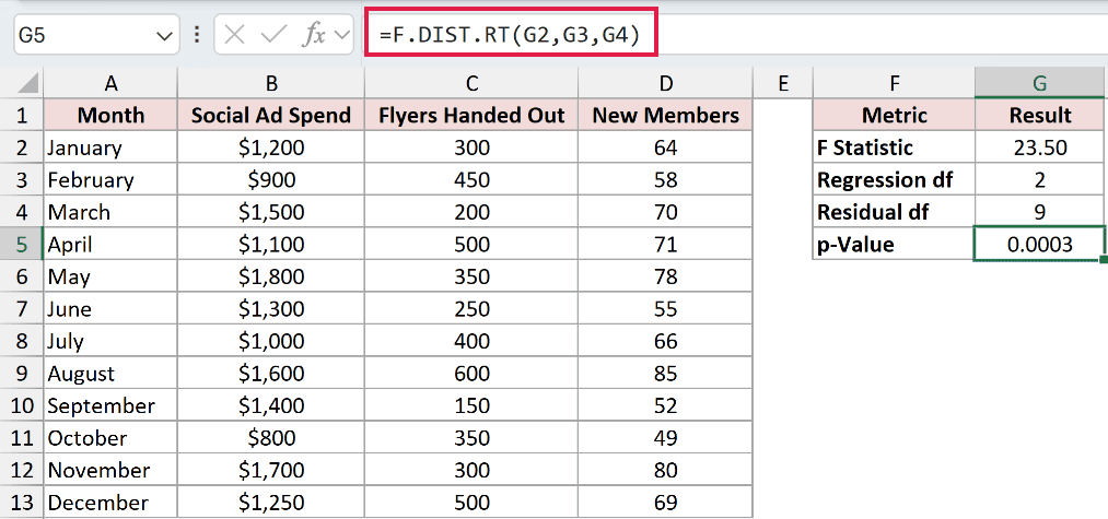
F.DIST.RT returns approximately 0.00026762, displayed as 0.0003. This is the value called Significance F in the Data Analysis ToolPak’s Regression output.
At a 0.05 significance level, the overall regression is significant. We reject the hypothesis that both predictor coefficients are zero.
Pro Tip: A significant overall F-test does not establish that both predictors are individually significant or that advertising causes signups. Interpret it alongside regression assumptions and individual coefficient tests.
Tips & Common Mistakes
- Keep the degrees of freedom in order. The first belongs to the numerator of the F statistic; the second belongs to the denominator.
- Match the tail to the question. ANOVA and overall regression use the right-tail probability directly. A two-sided variance comparison needs a two-tailed p-value.
- Check invalid inputs. Nonnumeric arguments return #VALUE!. Negative x or degrees of freedom below 1 return #NUM!. Noninteger degrees of freedom are truncated.
- Leave room for spilled results. Blocked output cells can cause #SPILL!. An implicit-intersection operator can reduce range input to one value instead of returning the full list.
- Check function availability. F.DIST.RT is available in Excel 2010 and later.
- Check spill support. Example 1 needs Excel 2021, Excel 2024 or Microsoft 365. In earlier versions, use row formulas and fill down.
- Distinguish related functions. F.DIST with TRUE returns the left-tail cumulative probability. Subtracting it from 1 gives the corresponding right tail. FDIST is the older name for F.DIST.RT.
- Compare without rounding. Use the underlying p-value for decisions, even when the cell displays only four decimal places.
- Use a cutoff when needed. F.INV.RT provides a right-tail critical value for comparing your F statistic with a threshold.
Other Excel articles you may also like:
