
The INTRATE function in Excel returns the annualized simple interest rate on a security you pay for upfront and receive money from at maturity.
Think of a discount note: you pay less than its maturity value, and the difference is your gain. INTRATE measures that gain against the amount you invested.
It also adjusts for the holding period and day-count method. The result is a simple annual rate, so it doesn’t assume that earnings compound.
I’ll show you how to compare investments, choose a day-count basis, and distinguish INTRATE from discount rates and compound annual returns.
INTRATE Function Syntax in Excel
INTRATE takes the purchase and maturity details, plus an optional day-count basis:
=INTRATE(settlement, maturity, investment, redemption, [basis])
- settlement (required): The date you pay for the security.
- maturity (required): The date the security pays out. It must be later than settlement.
- investment (required): The amount you pay. Enter a positive amount.
- redemption (required): The amount received at maturity. This must also be positive, even when you receive less than you invested.
- basis (optional): The day-count method used to annualize the return. Omitting it selects US (NASD) 30/360.
The available basis codes are:
- 0: US (NASD) 30/360. This is the default.
- 1: Actual/actual.
- 2: Actual/360.
- 3: Actual/365.
- 4: European 30/360.
The calculation divides the gain by the investment, then scales it to an annual rate using the selected day-count method.
When to Use INTRATE Function
- Calculate the annualized return on a discount note held until maturity.
- Compare simple annual rates for investments with different amounts and holding periods.
- Check how a security’s quoted day-count basis affects its rate.
- Calculate a simple annualized return from purchase cost and early-sale proceeds when there are no intervening payments.
Example 1: Calculate a Discount Note’s Annual Rate
Let’s start with a note that pays out at maturity.
Below is the dataset, with settlement and maturity dates, invested and maturity amounts, and a day-count basis. The labelled Interest Rate cell will hold the answer.
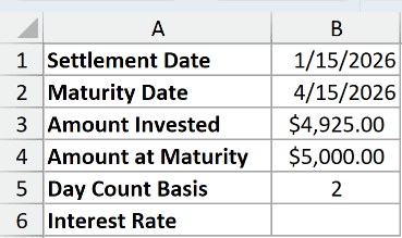
We want the annualized simple rate for this note in B6.
Here is the formula:
=INTRATE(B1,B2,B3,B4,B5)
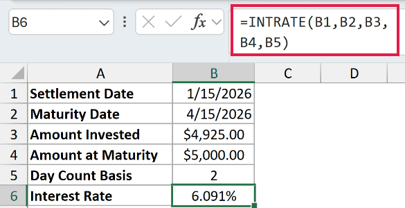
The formula returns 6.091%. It uses the $4,925.00 investment, the $5,000.00 maturity amount, and the dates in B1:B2.
Basis 2 means actual/360. Excel uses the actual holding period and a 360-day year to annualize the gain relative to the investment.
The rate expresses this shorter holding period’s return on an annual basis.
Pro Tip: Format the result as a percentage. Percentage formatting changes how the rate looks, without changing the underlying calculation.
Example 2: Compare Different Short-Term Investments
A larger dollar gain doesn’t necessarily mean a higher annual rate.
Below is the dataset, listing investments, maturity dates, amounts paid, and maturity amounts. Column E will hold annual rates; the side card contains settlement and basis inputs.

We want to compare each investment’s annualized simple rate using the same settlement date and basis.
Enter this formula in E2, then copy it down through E5:
=INTRATE($H$2,B2,C2,D2,$H$3)

The dollar signs keep H2 and H3 fixed. The maturity date and amounts change with each row, so this is a copied-down calculation.
The displayed rates are:
- 13-Week T-Bill: 4.805%.
- 26-Week T-Bill: 4.864%.
- 60-Day Commercial Paper: 4.351%.
- 120-Day Discount Note: 4.260%.
The discount note has the largest gap between purchase cost and maturity value, but the lowest annual rate. The longer T-bill has the highest rate here.
Example 3: Compare Day-Count Bases
Now let’s keep the note unchanged and vary only the basis.
Below is the dataset, with basis codes and method names in columns A:B, a result column C, and the note’s dates and amounts in E:F.
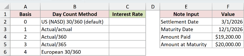
We want to see how each day-count method changes the same note’s annualized rate.
Enter this formula in C2, then copy it down through C6:
=INTRATE($F$2,$F$3,$F$4,$F$5,A2)
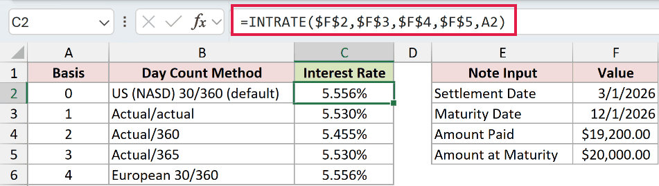
The locked references keep the note inputs unchanged. Only the basis reference moves as you copy the formula down.
US and European 30/360 both return 5.556%. Actual/actual and actual/365 both return 5.530%, while actual/360 returns 5.455%.
Different basis codes can agree for a particular date interval.
Pro Tip: Leaving basis out selects US (NASD) 30/360. Choose the method specified for the security instead of treating the omitted argument as a neutral setting.
Example 4: Compare INTRATE, YIELDDISC, and DISC
YIELDDISC calculates a discounted security’s annual yield from its price per $100 face value. We’ll compare that yield with INTRATE’s rate based on the actual amount invested.
DISC calculates a security’s annual discount rate using its maturity value. Comparing it with INTRATE shows how measuring the gain against different amounts changes the rate.
Below is the dataset, containing the bill’s dates, dollar amounts, quoted price, and basis. Labelled cells beneath the inputs will show INTRATE and the YIELDDISC and DISC comparisons.
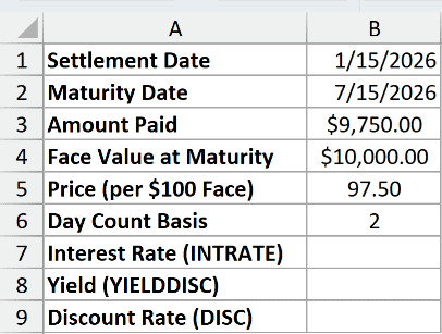
We want to compare the return on money invested with the bill’s yield and discount rate.
Start with INTRATE in B7:
=INTRATE(B1,B2,B3,B4,B6)
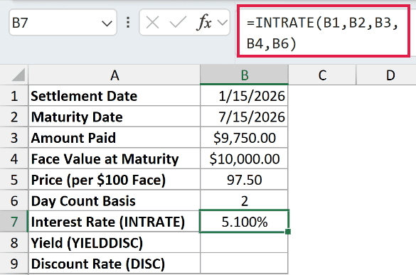
INTRATE returns 5.100%, using the $9,750.00 purchase cost and $10,000.00 maturity value.
For the YIELDDISC comparison in B8, use:
=YIELDDISC(B1,B2,B5,100,B6)
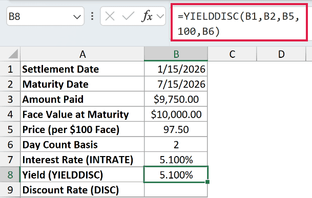
YIELDDISC also returns 5.100%. It uses the quoted price of 97.50 per $100 face value, with redemption entered directly as 100.
The price ratio and day-count basis match, so the yield matches INTRATE’s rate.
To compare discount rates, enter DISC in B9:
=DISC(B1,B2,B3,B4,B6)
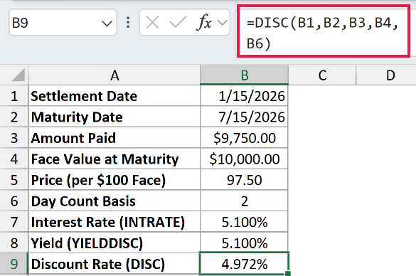
DISC returns 4.972%. It divides the gain by the maturity value, whereas INTRATE divides it by the amount invested.
That larger denominator makes the discount rate lower on this bill.
Example 5: Calculate Returns From an Early Sale
You can also use the actual exit date and proceeds to measure a holding period that ends before maturity.
Below is the dataset, listing sale scenarios, dates, and proceeds, with column D reserved for returns. The purchase card holds the original date, cost, and basis.

We want each scenario’s simple annualized return, including the sale at a loss.
Enter this formula in D2, then copy it down through D5:
=INTRATE($G$2,B2,$G$3,C2,$G$4)
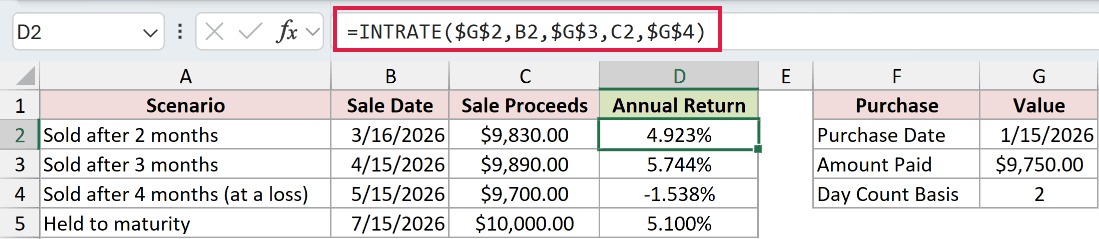
The sale date fills the maturity argument, and sale proceeds fill redemption. The purchase date, cost, and basis stay fixed as the formula is copied down.
The first sale returns 4.923%, and the next returns 5.744%. Each row represents a separate possible sale of the same investment.
The loss scenario returns -1.538% because the $9,700.00 proceeds are below the $9,750.00 purchase cost. A negative return is valid here.
The held-to-maturity scenario returns 5.100%, matching the previous example. It deliberately uses the same bill, purchase cost, and maturity payout.
Example 6: Compare Simple and Compound Annual Rates
For a longer holding period, the distinction between simple and compound returns matters.
Below is the dataset, with purchase and maturity details, basis, and typed Years Held input. The labelled result cells will hold INTRATE and the compound-rate comparison.
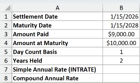
We want to compare the simple annual rate with the compound annual rate for this same note.
Enter INTRATE in B7:
=INTRATE(B1,B2,B3,B4,B5)
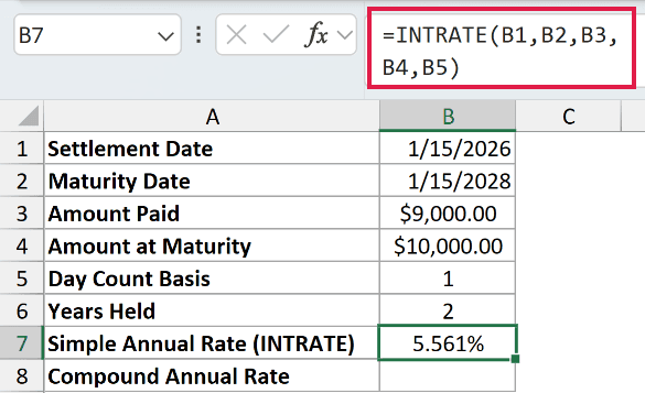
INTRATE returns 5.561% for the $9,000.00 investment growing to $10,000.00. It annualizes the gain using actual/actual, without compounding it.
To calculate the compound annual rate in B8, enter:
=(B4/B3)^(1/B6)-1
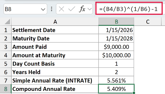
The compound formula returns 5.409%. It finds the constant yearly growth rate that connects the starting and ending amounts over the years in B6.
Here, B6 contains the typed input 2. The compound formula uses that holding period; INTRATE uses the dates and day-count basis instead.
Use the compound formula when you need a compound annual growth rate.
Example 7: Calculate Rates Across Purchase Prices
Changing the purchase price changes your return even when the final payout stays the same.
Below is the dataset, with purchase prices in column A and a result column B. The side card contains the note’s dates, maturity amount, and basis.
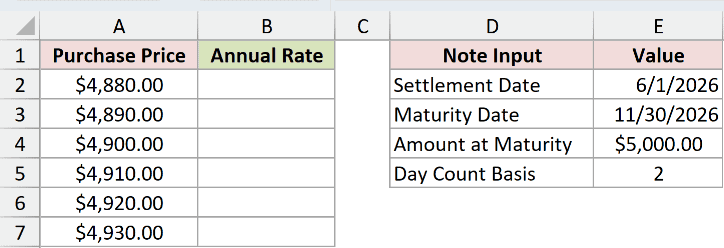
We want a rate for every purchase price from a single formula.
Enter this formula in B2:
=INTRATE(E2,E3,A2:A7+0,E4,E5)
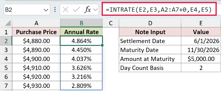
The +0 converts the price range into a numeric array that INTRATE can process. The formula spills its results into B2:B7.
This spill works in Excel 2021, Excel 2024, and Microsoft 365. In Excel 2019 and earlier, use a per-row calculation copied down instead.
At $4,880.00, the annual rate is 4.864%. At $4,930.00, it falls to 2.809%, because you pay more for the same maturity amount.
The intermediate prices return 4.450%, 4.037%, 3.626%, and 3.216%, in worksheet order.
Example 8: Identify Invalid Inputs
Invalid dates, amounts, or basis codes can produce errors.
Below is the dataset, with a valid case followed by deliberately invalid dates, an amount, and a basis. Column G will show each calculation’s result or error.

We want to see which inputs fail and what needs correcting in each row.
Enter this formula in G2, then copy it down through G7:
=INTRATE(B2,C2,D2,E2,F2)
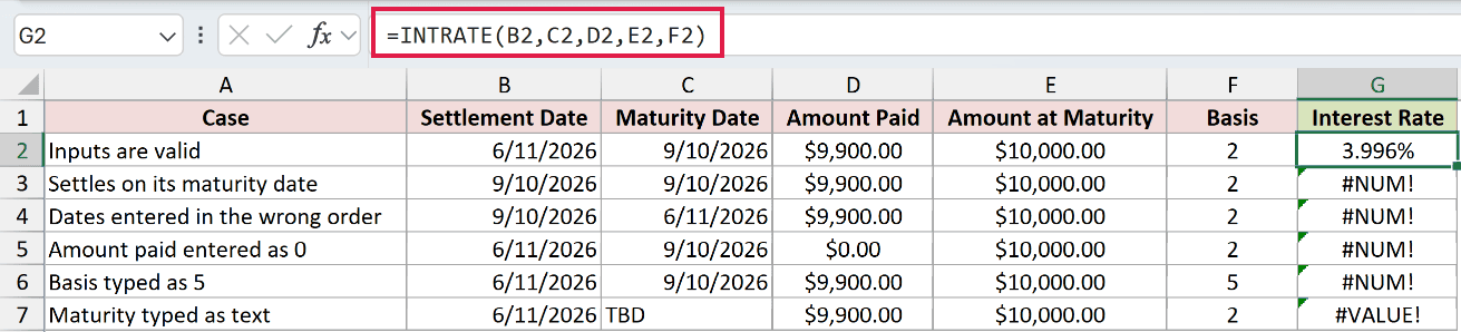
The valid row returns 3.996%. The remaining rows demonstrate errors on purpose:
- G3 returns
#NUM!: Settlement equals maturity. Correct the dates so settlement comes before maturity. - G4 returns
#NUM!: The dates are reversed. Put the earlier settlement date and later maturity date in their proper columns. - G5 returns
#NUM!: The amount paid is $0.00. Enter the positive purchase cost. - G6 returns
#NUM!: Basis is5, which isn’t supported. Select the appropriate code from0through4. - G7 returns
#VALUE!: The maturity cell containsTBD, which Excel can’t read as a date. Replace it with the actual maturity date.
Fix the underlying input rather than hiding these errors. Otherwise, the worksheet can look complete while the rate is still missing.
Tips & Common Mistakes
- Keep both amounts positive. A zero or negative investment or redemption returns
#NUM!. To represent a loss, enter positive proceeds below the positive purchase cost. - Check dates before changing the formula. Recognizable text dates can work, but unreadable text returns
#VALUE!. Date cells avoid dependence on how a text date is interpreted. - Use whole-number basis codes. Excel truncates a fractional basis:
1.9is treated as1. That can conceal a typing error. - Time values don’t add precision. INTRATE truncates the time portion of settlement and maturity, so this isn’t an intraday return calculation.
- Match the rate definition. INTRATE measures simple annual return on invested money; DISC measures discount relative to redemption. Neither replaces the compound comparison shown above.
Before comparing quoted rates, check that they use the same day-count method and the same definition of return.
Related Excel Functions / Articles:
