
The LEFTB function in Excel returns text from the beginning of a value, using a byte count that depends on your editing language settings.
On an English setup, LEFTB behaves like LEFT. You can extract prefixes from codes or shorten labels, but the B doesn’t automatically make it a universal byte counter.
An extracted year can look correct but still be text. That distinction matters when you use it in a calculation.
LEFTB Function Syntax in Excel
LEFTB takes the source text and an optional length:
=LEFTB(text, [num_bytes])
- text (required): The text or cell reference you want to extract from.
- num_bytes (optional): How much to keep from the beginning. When omitted, it defaults to 1.
Microsoft has deprecated LEFTB and recommends LEFT. LEFTB still works and returns the results shown here.
LEFTB counts double-byte characters as 2 only when a DBCS language, such as Japanese, Chinese, or Korean, is enabled and set as the default editing language.
DBCS means double-byte character set. On other setups, LEFTB counts characters like LEFT. All worked results below use an English setup.
When to Use LEFTB Function
- Extract a fixed prefix from flight numbers or account codes.
- Create filing letters from vendor names.
- Shorten labels to a fixed width and clean trailing spaces.
- Maintain extraction formulas in workbooks that use byte-based text functions.
Example 1: Extract Airline Codes From Flight Numbers
These flight numbers begin with an airline code.
Below is the dataset. Columns A and B contain flight numbers and routes, while column C has the Airline Code header and empty result cells.
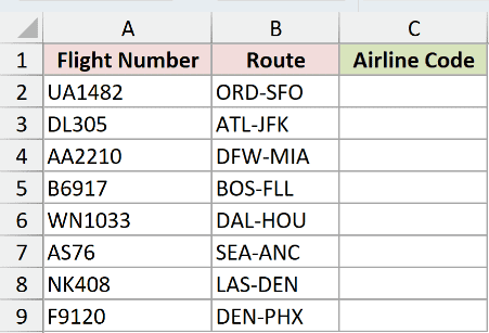
We want to extract the airline prefix from each flight number.
Enter this formula in C2:
=LEFTB(A2:A9,2)
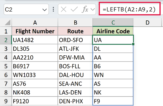
The formula spills into C2:C9. It returns “UA” for “UA1482”, “DL” for “DL305”, and “B6” for “B6917”.
LEFTB takes the specified length regardless of whether the prefix contains letters or digits. It doesn’t search for the first number.
Range formulas spill in Excel 2021, Excel 2024, and Microsoft 365. In Excel 2019 and earlier, use a per-row version and copy it down.
Example 2: Get Each Vendor’s Filing Letter
You can leave out the length when you only need the beginning letter.
Below is the dataset. Column A lists vendor names, and column B has a File Under header with empty cells for the filing letters.
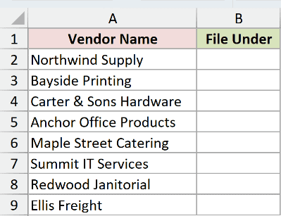
We want a filing letter for each vendor without specifying the length argument.
Enter this formula in B2:
=LEFTB(A2:A9)
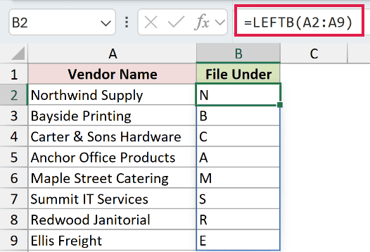
The results spill into B2:B9. “Northwind Supply” returns “N”, “Bayside Printing” returns “B”, and “Anchor Office Products” returns “A”.
Leaving out num_bytes uses the default of 1. On this English setup, that means the first character of each name.
Example 3: Shorten and Clean Receipt Labels
A fixed-width cut can leave a space at the end of a label.
Below is the dataset. Column A contains item names; columns B and C have headers and empty cells for untrimmed and clean receipt labels.
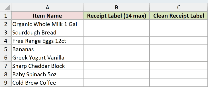
We want shortened receipt labels, then a clean version without trailing spaces.
First, enter the untrimmed comparison in B2:
=LEFTB(A2:A9,14)
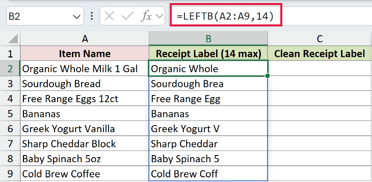
This comparison spills into B2:B9. B2 contains “Organic Whole ” and B7 contains “Sharp Cheddar “, each with a trailing space before the closing quote.
Now enter the clean version in C2:
=TRIM(LEFTB(A2:A9,14))
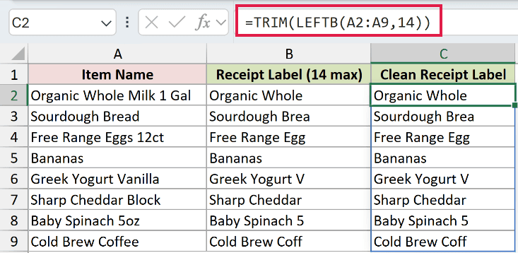
The clean labels spill into C2:C9. C2 returns “Organic Whole”, and C7 returns “Sharp Cheddar” after TRIM removes the trailing spaces.
“Bananas” stays “Bananas” in both columns. Asking for more than the available text returns the whole entry without adding padding.
LEFTB can cut through a word. TRIM cleans spaces around the extracted text; it doesn’t restore letters removed by the cut.
Example 4: Turn Extracted Digits Into Numbers
Digits extracted from a numeric code still come back as text.
Below is the dataset. Column A holds production codes, while columns B and C have headers and empty cells for text years and numeric years.
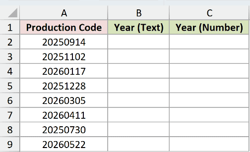
We want the year prefix from each production code, converted to a number when needed.
Enter the text-result formula in B2:
=LEFTB(A2:A9,4)
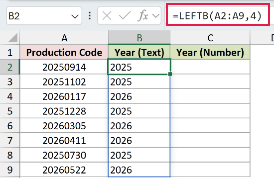
The text results spill into B2:B9. The code “20250914” returns “2025”, shown left-aligned in the Year (Text) comparison column.
Enter the numeric version in C2:
=VALUE(LEFTB(A2:A9,4))
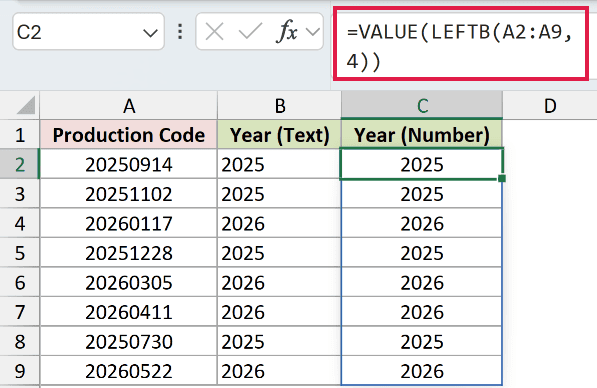
This formula spills into C2:C9. C2 also displays “2025”, but VALUE converts the extracted text into a number.
The matching digits can hide that difference. Keep the text form for a text identifier; use the numeric form when the receiving calculation or lookup needs numbers.
Example 5: Extract Several Account Prefixes Together
Account numbers can encode several levels of grouping in their prefixes.
Below is the dataset. Columns A and B list account numbers and names; columns C through E have Class, Group, and Subgroup headers above empty cells.
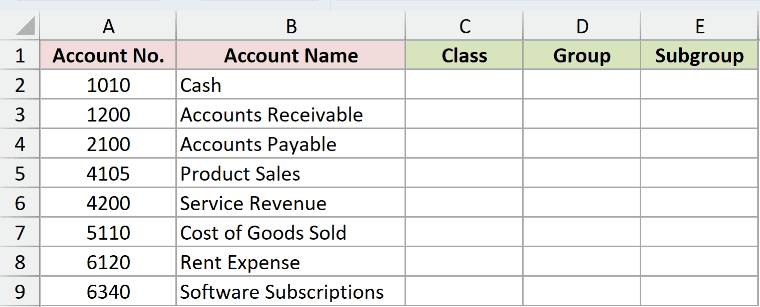
We want the class, group, and subgroup prefixes for each account in the same result grid.
Enter this formula in C2:
=LEFTB(A2:A9,{1,2,3})
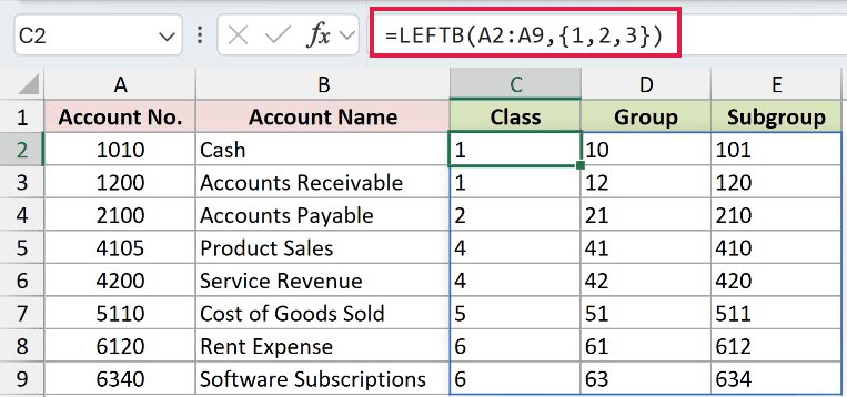
The formula spills across and down into C2:E9. The horizontal array {1,2,3} requests progressively longer prefixes for every account in the vertical source range.
Cash, account “1010”, returns “1”, “10”, and “101”. Product Sales, account “4105”, returns “4”, “41”, and “410”.
These prefixes are text, just like the unconverted results in the previous example.
Example 6: Avoid Extracting Date Serial Digits
Real Excel dates need a different approach from numeric production codes.
Below is the dataset. Column A contains order dates. Columns B and C have headers and empty cells for the direct-LEFTB mistake and corrected year-month keys.
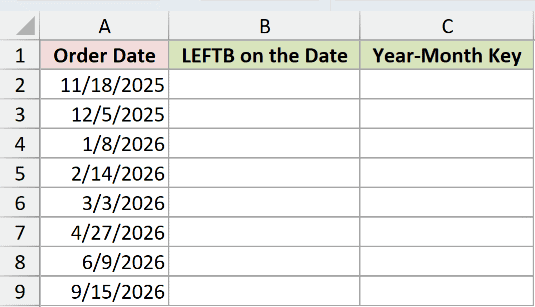
We want a year-month key from each date.
This formula in B2 demonstrates the wrong approach:
=LEFTB(A2:A9,4)
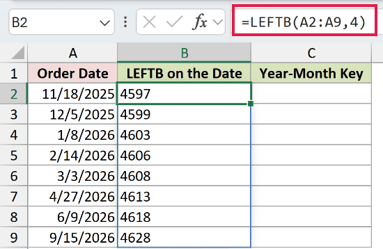
The mistaken results spill into B2:B9. For “11/18/2025”, B2 returns “4597”. For “9/15/2026”, B9 returns “4628”.
Those are digits from the stored date serials. LEFTB doesn’t read the date formatting you see on the worksheet.
Enter the correction in C2:
=LEFTB(TEXT(A2:A9,"yyyy-mm-dd"),7)
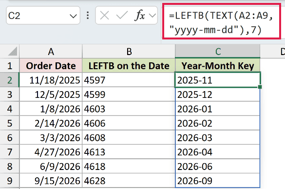
The corrected keys spill into C2:C9. C2 returns “2025-11”, and C9 returns “2026-09”.
TEXT first turns each date into text using yyyy-mm-dd. LEFTB then extracts the year-month portion from that formatted text.
Pro Tip: For a year-month key alone, TEXT with the yyyy-mm format is more direct. The example shows why formatting must happen before LEFTB extracts from a date.
Tips & Common Mistakes
- A
num_bytesvalue of 0 returns empty text. A negative value returns#VALUE!, while a decimal length is truncated. - LEFT is the everyday choice for character-based extraction. Use LEFTB when the workbook specifically needs its language-dependent byte behavior.
- FINDB returns the byte position of one piece of text inside another. Use that position to work out LEFTB’s
num_bytesso the extraction length uses bytes too. Mixing character positions and byte lengths can extract the wrong number of characters under DBCS settings. - Leave the intended spill area empty. A blocked result range causes
#SPILL!. - Check the source value’s type before extracting. A numeric code, a text identifier, and a formatted date can look similar while requiring different treatment.
A prefix can be a filing letter or an account grouping, depending on the length you keep. The examples above show both uses with whole columns.
Other Excel articles you may also like:
