
An attendance tracker in Excel lets you mark who was present, late, absent, sick, or excused each day, then turns those marks into totals and an attendance percentage.
Setting up the grid is easy. The calendar around it takes more thought.
A good tracker has to know which days are weekends, which days are holidays, and how many working days the month really has.
Otherwise the totals look right but can’t be trusted.
In this article, I’ll show you how to build a monthly attendance sheet that sets up its own dates from one cell and shades weekends and holidays.
You’ll also add drop-downs and color codes for the attendance marks.
Then I’ll show you how to count each code, flag missing entries, calculate attendance percentages, and protect the sheet so people can only fill in their codes.
Using the Free Attendance Tracker Template
If you just want a tracker that works, download the file above. It has everything from this article already set up.
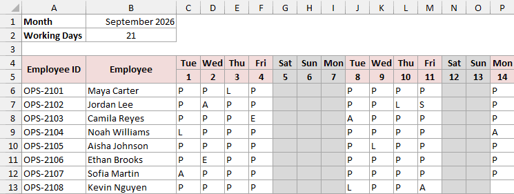
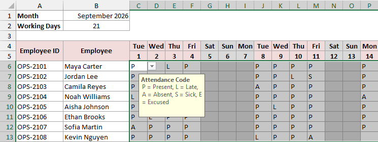
Below is the finished tracker on the Attendance sheet. It covers September 2026 for a team of eight, with one column per day and a summary on the right.

Here is how to reuse it for your own team:
- Type the first day of your month in cell B1, like 10/1/2026. The dates, weekday names, and shading all update.
- Replace the IDs and names in A6:B13 with your own people.
- Select C6:AG13 and press Delete to clear the September codes.
- Add your holidays to the Holidays sheet, one date per row.
If you’d rather start from one of Microsoft’s designs, Excel has its own attendance templates. Click File > New, type attendance in the search box, and press Enter.
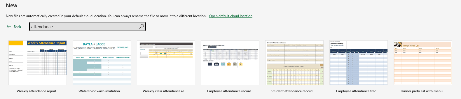
Pick a template, click Create, and replace its sample names and dates with yours.
The rest of this article shows you how to build the tracker yourself, one step at a time. It’s also handy if you want to change how the download works.
Step 1: Setting Up the Month and the Holiday List
The whole tracker runs off one date. Everything else, from the date headers to the working-day count, is calculated from it.
In cell B1 on the Attendance sheet, I typed 9/1/2026, the first day of the month I want to track.
I formatted it with the custom format mmmm yyyy so it reads September 2026.
Next, I need a list of holidays so Excel knows which weekdays are not working days.
Below I have a separate sheet called Holidays, with the holiday dates in column A and their names in column B.
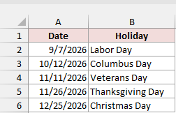
Here are the steps to give the holiday dates a name, so formulas can refer to them easily:
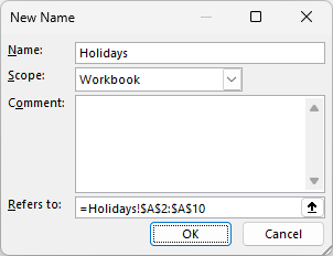
- On the Holidays sheet, select A2:A10. This covers the five holidays plus a few empty rows for ones you add later.
- Go to Formulas > Define Name. In the New Name dialog box, type Holidays in the Name box, check that Refers to shows =Holidays!$A$2:$A$10, and click OK.
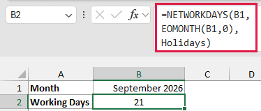
Now I can count the working days in the month. Here is the formula I entered in cell B2 on the Attendance sheet:
=NETWORKDAYS(B1,EOMONTH(B1,0),Holidays)
How does this formula work?
EOMONTH(B1,0) returns the last day of the month in B1, which is September 30, 2026.
NETWORKDAYS then counts the weekdays from B1 to that date and skips any date in the Holidays list.
September 2026 has 22 weekdays. Labor Day falls on Monday, September 7, so the result is 21 working days.
Step 2: Adding the Names and the Dates
Now let’s add the people and a column for every day of the month.
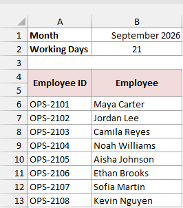
Below I have the month and working days in A1:B2, and the employee IDs and names in A6:B13.
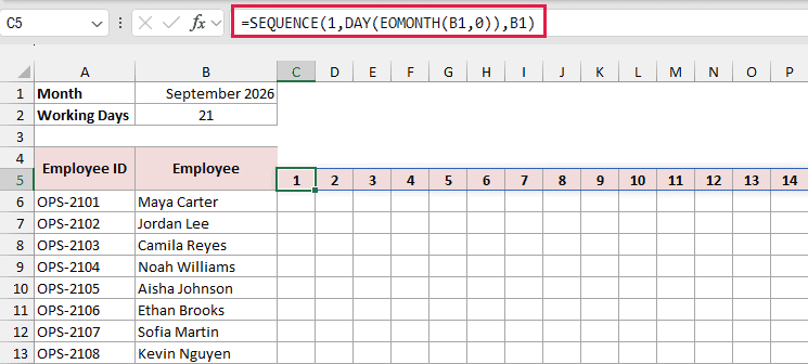
I want one column per day, starting in C5, with real dates rather than typed labels. Here is the formula I entered in cell C5:
=SEQUENCE(1,DAY(EOMONTH(B1,0)),B1)
How does this formula work?
DAY(EOMONTH(B1,0)) returns the number of days in the month, which is 30 for September.
The SEQUENCE function uses that 30 as the number of columns. It returns one row of 30 dates, starting at B1 and going up by 1 each time.
The formula spills across to AF5 automatically.
Since these are real dates, I gave C5:AG5 the custom format d, so each cell shows just the day number.
I also made the day columns narrow so the whole month fits on screen.
Change B1 to October and the dates run to 31 in column AG. Change it to February and they stop at 28.
Note: SEQUENCE and the spill behavior need Excel 365, Excel 2021, or a later version. In older versions, type =B1 in C5, enter =IF(C5=””,””,IF(C5+1>EOMONTH($B$1,0),””,C5+1)) in D5, and copy it across to AG5.
Step 3: Showing the Weekday Names
Day numbers alone make it hard to spot the weekends, so I’ll add the weekday name above each date.
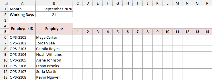
Below I have the tracker with the day numbers in row 5 and an empty row 4 above them.
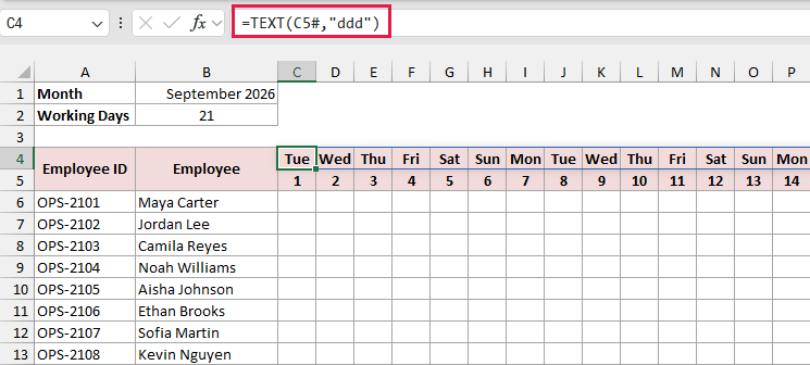
Here is the formula I entered in cell C4:
=TEXT(C5#,"ddd")
How does this formula work?
C5# refers to the whole spilled range of dates that starts in C5. So if the month has 31 days, the weekday row grows to 31 cells too.
TEXT with the “ddd” format returns the short day name for each date, like Tue for September 1, 2026.
Note: The # reference needs Excel 365, Excel 2021, or later. In older versions, enter =TEXT(C5,”ddd”) in C4 and copy it across to AG4.
Step 4: Shading Weekends and Holidays
Nobody should be marking attendance on a Saturday or on Labor Day. Shading those columns gray makes them easy to skip.
I’ll use conditional formatting with a formula, so the shading moves on its own when you change the month.
Here are the steps to highlight the weekends and holidays:
- Select C4:AG13. This covers the weekday row, the dates, and all the attendance cells.
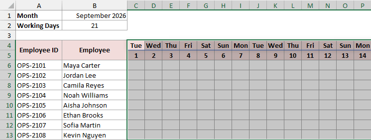
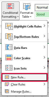
- Go to Home > Conditional Formatting > New Rule.
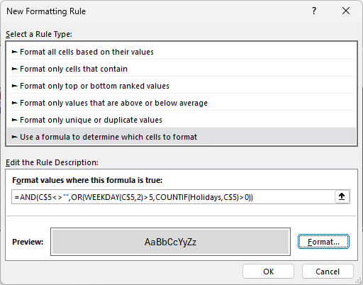
- Choose Use a formula to determine which cells to format, and enter the formula below in the box. Click Format, pick a light gray fill on the Fill tab, and click OK.
=AND(C$5<>"",OR(WEEKDAY(C$5,2)>5,COUNTIF(Holidays,C$5)>0))
- Click OK to apply the rule.
The weekend columns and the Labor Day column now turn gray.
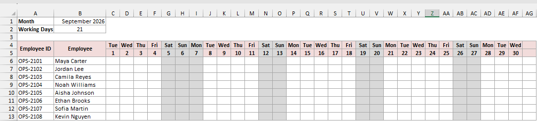
How does this formula work?
WEEKDAY(C$5,2) numbers the days from 1 for Monday to 7 for Sunday, so anything above 5 is a Saturday or Sunday.
COUNTIF(Holidays,C$5)>0 checks whether the date is on the holiday list. OR shades the column if either test is true.
The C$5<>”” part stops the rule from shading column AG in months with fewer than 31 days.
The dollar sign before 5 makes every row in the column check the date in row 5.
Step 5: Highlighting Today’s Date
When you fill in the tracker every day, it helps to see today’s column at a glance. Another conditional formatting rule does this.
Here are the steps to highlight today’s date:
- Select C4:AG5, the weekday and date rows.
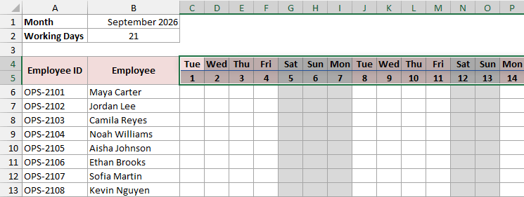
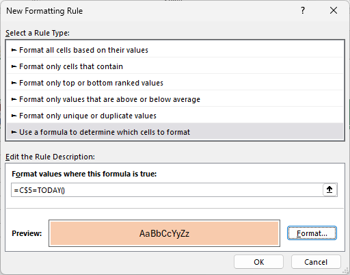
- Go to Home > Conditional Formatting > New Rule, choose Use a formula to determine which cells to format, and enter the formula below. Click Format, pick an orange fill, and click OK twice.
=C$5=TODAY()
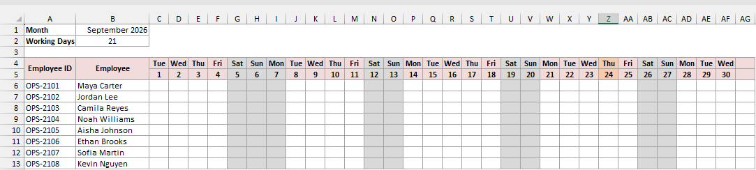
Today’s day and date now stand out in orange. The rule only lights up when the month in B1 is the current month.
Step 6: Adding a Drop-Down for the Codes
Typed entries are where most attendance sheets go wrong. One person types P, another types Present, and the counts break.
I’ll use these five codes: P for Present, L for Late, A for Absent, S for Sick, and E for Excused.
Here are the steps to add a drop-down list of the codes:
- Select C6:AG13, the cells where the codes go.
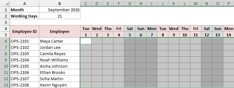
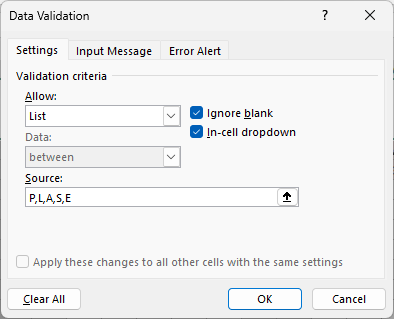
- Go to Data > Data Validation. On the Settings tab, choose List in the Allow box and type P,L,A,S,E in the Source box.
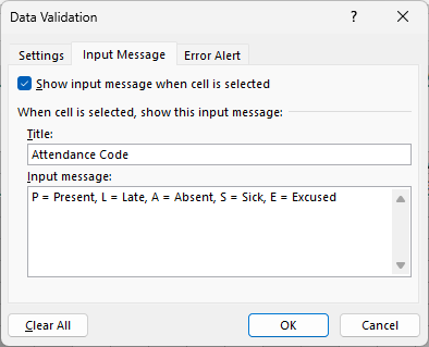
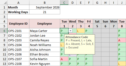
- Go to the Input Message tab. Type Attendance Code as the title and P = Present, L = Late, A = Absent, S = Sick, E = Excused as the message. Then click OK.
Now, when you click any attendance cell, a small arrow appears. Click it and pick a code from the list.
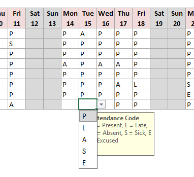
The input message also pops up when you select a cell, so nobody has to remember what S or E means.
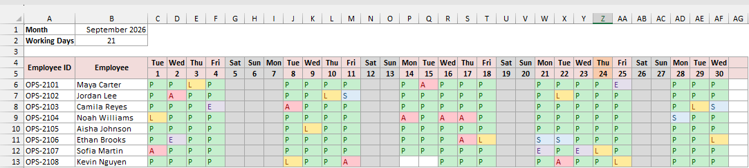
Below is the tracker after filling in the codes for September. Weekends and Labor Day stay empty.
Note: Data Validation only checks what people type. If someone pastes values into the grid, anything can get in, so check pasted data before you trust the totals.
Step 7: Color-Coding Each Code
With a whole month of letters in the grid, it’s hard to spot an absence. Colors fix that. Here, each code gets its own fill through conditional formatting.
Here are the steps to color-code the codes:
- Select C6:AG13, the attendance cells.
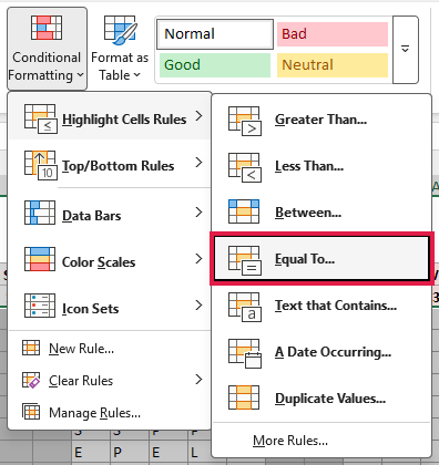
- Go to Home > Conditional Formatting > Highlight Cells Rules > Equal To.
- Type P in the box on the left, choose Green Fill with Dark Green Text on the right, and click OK.
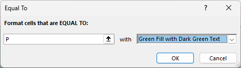
- Repeat Steps 2 and 3 for L with Yellow Fill with Dark Yellow Text, and for A with Light Red Fill with Dark Red Text.
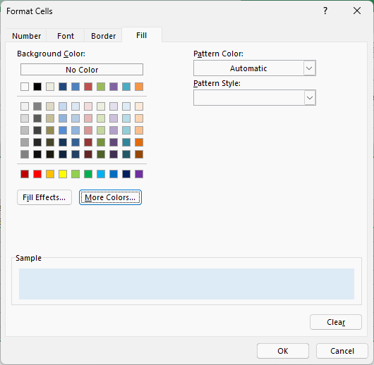
- For S and E, choose Custom Format in the right-hand drop-down. On the Fill tab, click More Colors, go to the Custom tab, and enter the hex code DDEBF7 for a light blue. Do the same for E with E4DFEC, a light purple. Then click OK to close each dialog.
Each code now has its own color, so absences and late days jump out right away.
Step 8: Counting Each Code With COUNTIF
Now for the totals. I want to know how many days each person was present, late, absent, sick, or excused.
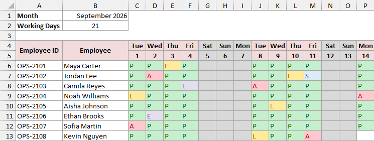
Below I have the filled-in, color-coded tracker. The totals go in columns AH to AL, right after the last day column.
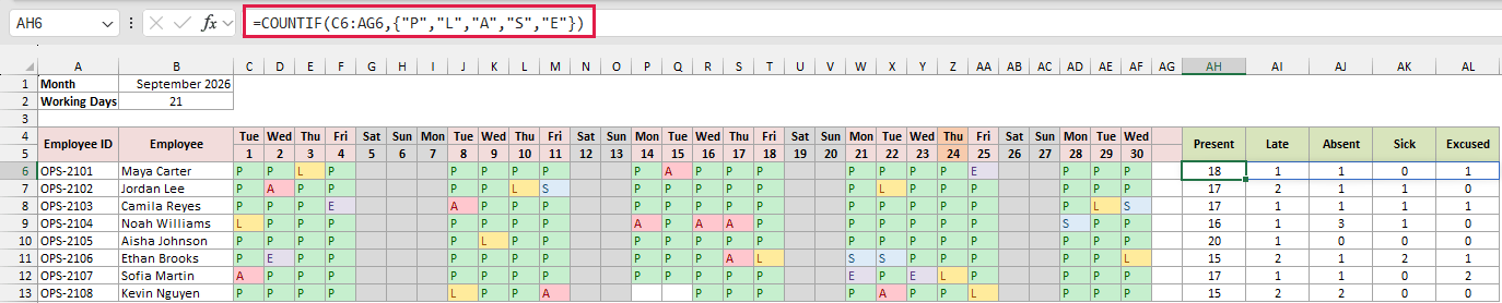
Here is the formula I entered in cell AH6 and then copied down to AH13:
=COUNTIF(C6:AG6,{"P","L","A","S","E"})
How does this formula work?
The part in curly brackets is an array constant with all five codes. COUNTIF counts each code separately in the person’s row, C6:AG6.
That gives five results, so the formula spills across AH6:AL6. For Maya Carter, it returns 18 Present, 1 Late, 1 Absent, 0 Sick, and 1 Excused.
Note: In Excel 2019 or older, the formula won’t spill. Use one COUNTIF per column instead, like =COUNTIF($C6:$AG6,”P”) in AH6 and =COUNTIF($C6:$AG6,”L”) in AI6, then copy them down.
Step 9: Checking for Missing Entries
A blank cell on a working day usually means someone forgot to record it. That quietly throws off the totals, so I’ll count the gaps.
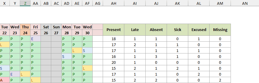
Below I have the tracker with the codes for September. Kevin Nguyen has no codes on September 14 and 15.
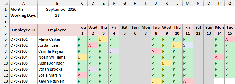
Here is the formula I entered in cell AM6 and copied down to AM13:
=$B$2-COUNTA(C6:AG6)

How does this formula work?
COUNTA counts the cells in the row that have a code.
B2 holds the 21 working days from Step 1, and the dollar signs keep it fixed as you copy down.
So the result is the number of working days with no code. Everyone shows 0 except Kevin Nguyen, who shows 2.
Step 10: Calculating the Attendance Percentage
The attendance percentage is present days plus late days, divided by the days that count. Which days count depends on your policy for sick and excused days.
Below I have the tracker with the counts and the missing-entry check.
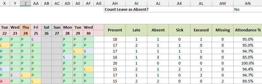
Next, I added a setting in AN1 called Count Leave as Absent?, set to No. I gave it a Yes/No drop-down with Data Validation, the same way as in Step 6.
Here is the formula I entered in cell AN6 and copied down to AN13:
=IFERROR((AH6+AI6)/(AH6+AI6+AJ6+IF($AN$1="Yes",AK6+AL6,0)),"")

How does this formula work?
AH6+AI6 adds the present and late days, so a late day still counts as attended.
The bottom part adds present, late, and absent days. If AN1 is Yes, it also adds the sick and excused days, so they count against the person.
For Maya Carter with AN1 set to No, that’s 19 divided by 20, or 95.0%. Switch AN1 to Yes and it drops to 19 out of 21, or 90.5%.
IFERROR returns a blank instead of a #DIV/0! error for a row with no codes yet. I formatted AN6:AN13 as a percentage with one decimal place.
Step 11: Adding a Team Summary
Individual percentages are useful, but a manager or teacher also wants the big picture. I’ll add a daily head count, a team average, and a flag for low attendance.
Below I have the tracker with each person’s attendance percentage in column AN.
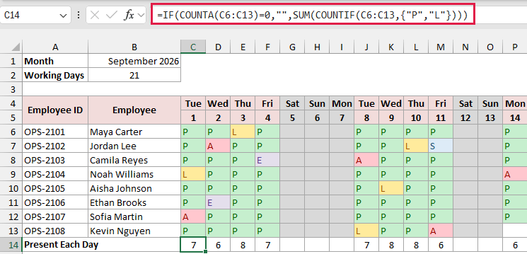
First, the head count. Here is the formula I entered in cell C14 and copied across to AG14:
=IF(COUNTA(C6:C13)=0,"",SUM(COUNTIF(C6:C13,{"P","L"})))
How does this formula work?
COUNTIF with {“P”,”L”} counts the present and late codes in that day’s column, and SUM adds the two counts together. On September 1, that’s 7 people.
If nobody has a code that day, like on a weekend, COUNTA returns 0 and the cell stays blank.
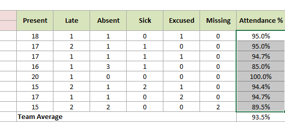
Next, the team average. Here is the formula I entered in cell AN14:
=AVERAGE(AN6:AN13)

It averages the eight percentages, which gives a team attendance of 93.5%.
Finally, I’ll highlight anyone below a target. I typed 90% in cell AN2, next to the label Flag Rates Below.
Here are the steps to flag low attendance:
- Select AN6:AN13, the attendance percentages.
- Go to Home > Conditional Formatting > New Rule, choose Use a formula to determine which cells to format, and enter the formula below. Click Format, pick a light red fill, and click OK twice.
=AND(AN6<>"",AN6<$AN$2)
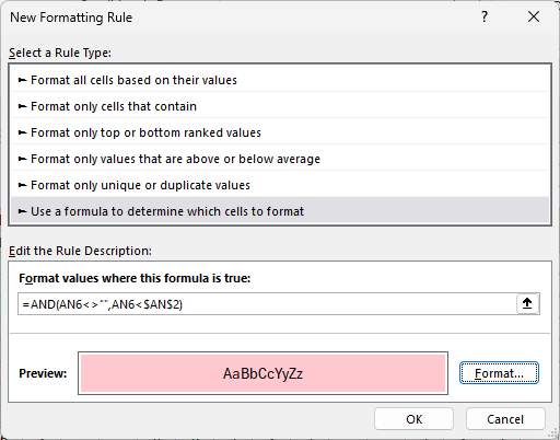
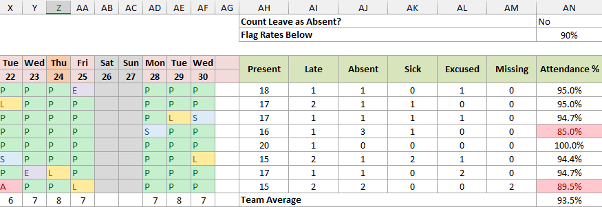
Noah Williams at 85.0% and Kevin Nguyen at 89.5% are now highlighted in red. Change AN2 and the flags update.
Step 12: Freezing the Names and Dates
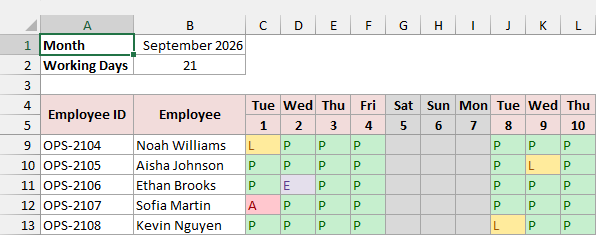
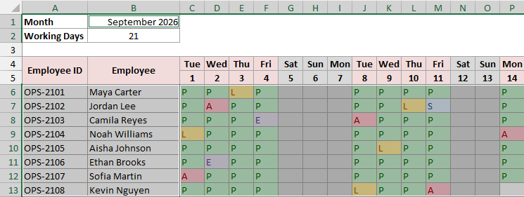
The tracker is 40 columns wide. Once you scroll to the end of the month, you lose sight of the names.
Freeze Panes keeps the names and the date rows in place while you scroll.
Here are the steps to freeze the names and dates:
- Click cell C6, the first attendance cell. Everything above it and to its left will stay visible.
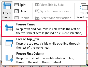
- Go to View > Freeze Panes > Freeze Panes.
Now, when you scroll right, columns A and B stay put. When you scroll down, the rows with the month, weekdays, and dates stay at the top.
Step 13: Protecting the Sheet
If other people fill in the tracker, it’s easy for someone to overwrite a formula by accident. Protecting the sheet keeps the formulas safe while leaving the code cells open.
By default, every cell is locked, but that only takes effect once the sheet is protected. So first, you unlock the cells people should be able to change.
Here are the steps to protect the sheet:
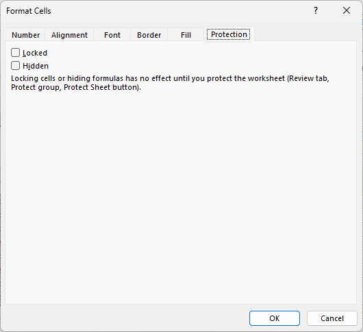
- Select C6:AG13. Then hold Ctrl and also select A6:B13, B1, and AN1:AN2, so the names and settings stay editable too.
- Press Ctrl + 1 (Cmd + 1 on a Mac) to open Format Cells. On the Protection tab, uncheck Locked and click OK.
- Go to Review > Protect Sheet. Enter a password if you want one, and click OK.
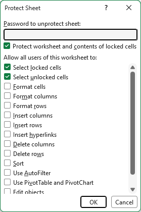
Now anyone can pick codes in the grid, but if they try to type over a formula, Excel stops them with a warning.
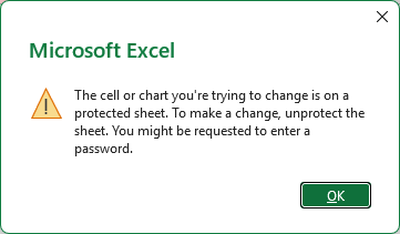
To make changes later, go to Review > Unprotect Sheet. The download above is not protected, so you can edit it right away.
Additional Notes About Attendance Trackers in Excel
- Stick to the five codes. The formulas count exact codes, so a typed word like Present won’t be counted anywhere.
- The tracker treats Saturday and Sunday as the weekend. If your team has a different work week, use NETWORKDAYS.INTL in B2 and change the WEEKDAY test in the Step 4 rule to match.
- The weekday names follow your Excel language settings, so TEXT with “ddd” may show them in your own language.
- The Holidays name covers A2:A10. If you need more than nine holidays, extend the range in Formulas > Name Manager.
- The attendance percentage only uses days that have a code. That keeps it accurate in the middle of a month, as long as the Missing column shows 0.
Frequently Asked Questions
How do I make an attendance sheet for students in Excel?
Use the same tracker.
Put student IDs and names in A6:B13, and list school holidays and breaks on the Holidays sheet so they’re shaded and left out of the working days.
How do I track half days in an Excel attendance sheet?
Add a code like H to the drop-down source and give it a color rule.
Then add 0.5*COUNTIF(C6:AG6,”H”) to the top of the percentage formula and COUNTIF(C6:AG6,”H”) to the bottom, so a half day counts as half attended.
How do I make a yearly attendance tracker in Excel?
Copy the Attendance sheet once for each month, name the copies Jan to Dec, and set B1 on each one.
Then add up any count across the year with a 3D reference like =SUM(Jan:Dec!AH6).
How do I add more people to the attendance tracker?
Insert new rows between row 6 and row 13, so every range and rule stretches to include them.
Then copy the formulas in AH:AN down into the new rows. If the sheet is protected, unprotect it first.
Conclusion
In this article, I showed you how to build an attendance tracker that sets up its own dates, uses drop-downs and color codes, and calculates the totals.
The quickest way to start is the free download. Change the month in B1, add your names, and you’re ready to go.
I hope you found this article helpful.
Other Excel articles you may also like:
