Slicers vs Filters in Excel (Differences and When to Use Each)

Slicers and filters in Excel do the same basic job. They hide the rows you don’t want so you can focus on the ones you do.

Where they differ is in how you use them and what they can do.

A slicer is a panel of buttons that sits on the sheet and shows what’s filtered at a glance. A filter is a drop-down arrow in a column header.

Neither one wins every time. Slicers are easier to click anfed read, but they can’t filter by a condition like “greater than 500” or “contains Bean”.

In this article, I’ll show you the same filter done both ways on a Table and a PivotTable.

Then I’ll compare them on conditions, multiple PivotTables, protected sheets, and Excel for the web.

Slicer vs Filter in Excel: Quick Comparison

Here’s how the two stack up side by side. Each row is covered with a worked example further down.

	Slicer	Filter drop-down
Works on	Excel Tables and PivotTables	Any range, Table, or PivotTable
How you filter	Click a button	Open a list and check boxes
Shows what’s filtered	Yes, the selected buttons are highlighted	Only a small funnel icon on the header
Several items at once	Ctrl + click, or the Multi-Select button	Check several boxes
Conditions (greater than, contains, top 10)	No	Yes
Search box	No	Yes
Dates	One button per date (use a Timeline for PivotTables)	Grouped by year, month, and day, plus date filters
Controls several PivotTables	Yes, with Report Connections	No, one PivotTable only
Space on the sheet	Takes up a block of cells	None
Protected sheet	Works if the slicer is unlocked and the right option is checked	Works if the right option is checked
Excel versions	PivotTables: Excel 2010 and later. Tables: Excel 2013 and later	Every version
Excel for the web	Use any slicer. Insert new ones for PivotTables only	Yes

If you want the basics of inserting and formatting slicers first, my guide on how to use slicers in Excel covers them step by step.

Filtering an Excel Table: Filter vs Slicer

Let me start with a Table, since that’s where most people first meet both tools.

Below I have a Table of 14 wholesale orders from a coffee roaster.

Each order has a date, the cafe that bought it, the cafe’s city, the roast, the bags sold, and the revenue.

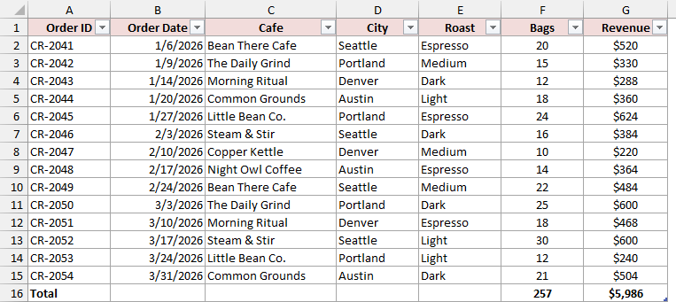
The Table has a Total Row at the bottom, which uses SUBTOTAL. That’s why the totals will change as we filter.

I want to show only the orders from Seattle.

Using the Filter Drop-Down

An Excel Table already has a filter arrow in every header, so there’s nothing to set up.

Here are the steps to filter the Table with the drop-down:

1. Click the filter arrow in the City header.

2. Uncheck (Select All), check Seattle, and click OK.

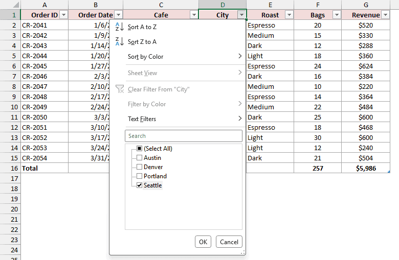
The Table now shows the four Seattle orders, and the Total Row shows $1,988.

Look at the City header. The arrow has turned into a small funnel icon. That icon is the only sign on the sheet that something is filtered.

Using a Slicer

Now let’s do the same thing with a slicer.

Here are the steps to add a slicer to the Table:

1. Select any cell in the Table.

2. Go to the Table Design tab and click Insert Slicer.

3. In the Insert Slicers dialog box, check City and click OK.

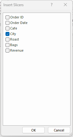
Excel adds a City slicer with one button per city. Click Seattle.

You get the same four orders and the same $1,988. The difference is that the highlighted Seattle button tells anyone looking at the sheet exactly what’s showing.

The slicer and the drop-down also share one filter. If you filter City with the drop-down, the slicer moves to match, and the reverse is true too.

Filtering a PivotTable: Filter vs Slicer

A PivotTable gives you the same choice, but the built-in filter works a little differently here.

Using a Report Filter

Below I have a PivotTable built from the same orders. It shows the revenue for each roast, and I’ve dragged City into the Filters area of the PivotTable Fields pane.

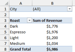
That puts a filter cell above the PivotTable. This is called a Report Filter, and it currently shows (All).

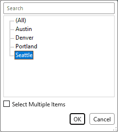
Here are the steps to show only Seattle:

1. Click the filter arrow in cell B1.

2. Select Seattle and click OK.

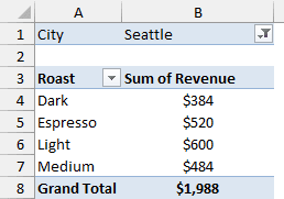
The PivotTable now shows only the Seattle revenue for each roast. Espresso is $520, Dark is $384, Medium is $484, and Light is $600, for a total of $1,988.

Using a Slicer

For the slicer version, I’ve built the same Revenue by Roast PivotTable without anything in the Filters area.

Here are the steps to filter it with a slicer:

1. Select any cell in the PivotTable.

2. Go to the PivotTable Analyze tab and click Insert Slicer.

3. Check City, click OK, and then click Seattle in the slicer.

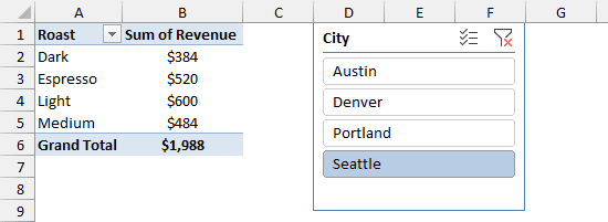
The numbers match the Report Filter exactly. Notice that City isn’t anywhere in the PivotTable’s layout.

A slicer can filter by any field in the data, even one the PivotTable doesn’t show. A Report Filter only works for a field you’ve put in the Filters area.

Key Differences Between Slicers and Filters

Both tools gave the same answer in every example so far. The differences show up once you go beyond picking one item.

Seeing What’s Filtered

This is where slicers pull ahead. With one city picked, a Report Filter at least shows its name in cell B1.

Pick two cities, though, and the Report Filter just says (Multiple Items). Below, Seattle and Portland are both selected, for a total of $3,782.

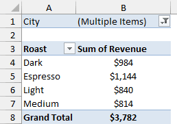
Anyone reading this report has to open the drop-down to find out which cities are in it. A Table’s drop-down filter is even quieter, with just the funnel icon.

Here’s the same filter with a slicer. You can see Seattle and Portland are in, and Austin and Denver are out.

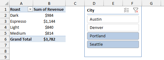
This is the main reason slicers work so well on reports that other people open. They don’t need to know how filters work to read the report.

Selecting Several Items

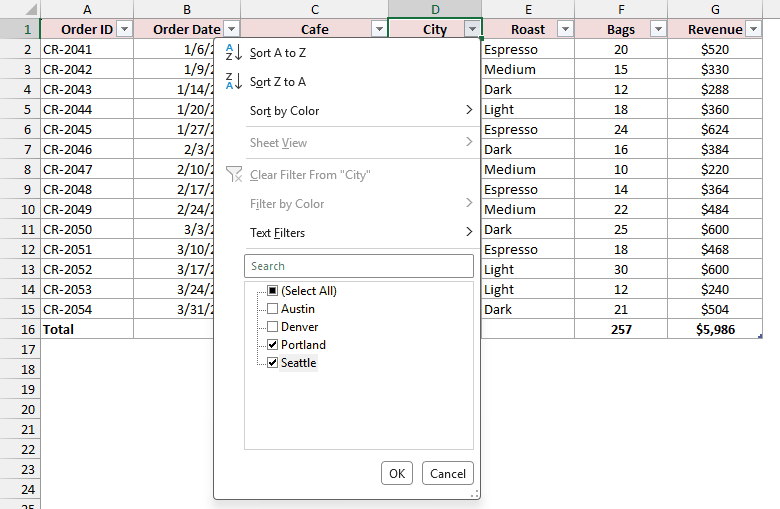
With a filter drop-down, you pick several items by checking their boxes.

Below, I’ve opened the City filter on the Table and left only Seattle and Portland checked.

With a slicer, you Ctrl + click each button you want.

You can also click the Multi-Select button at the top of the slicer (or press Alt + S), and then every click adds or removes one city.

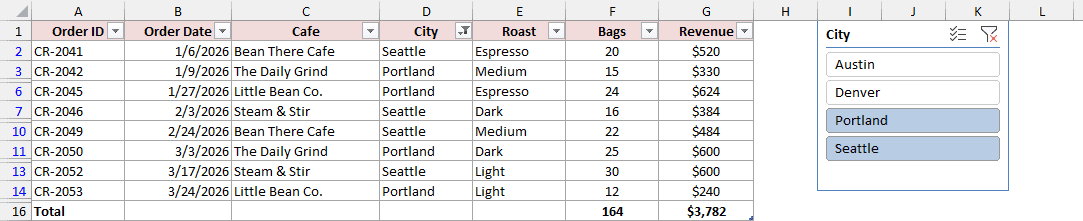
Both give you the same eight orders and $3,782.

For a Report Filter, you first need to check Select Multiple Items at the bottom of its drop-down, or it only lets you pick one.

Note: To clear a slicer, click the Clear Filter button in its top-right corner, or select the slicer and press Alt + C. To clear a drop-down filter, open it and choose Clear Filter From “City”.

Filtering by a Condition (Greater Than, Contains)

This is the biggest gap. A slicer can only show or hide items from its list. It has no way to say “revenue above $500” or “cafe names that contain Bean”.

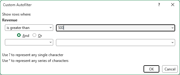
The filter drop-down can. On the Table, open the Revenue filter, go to Number Filters, and pick Greater Than.

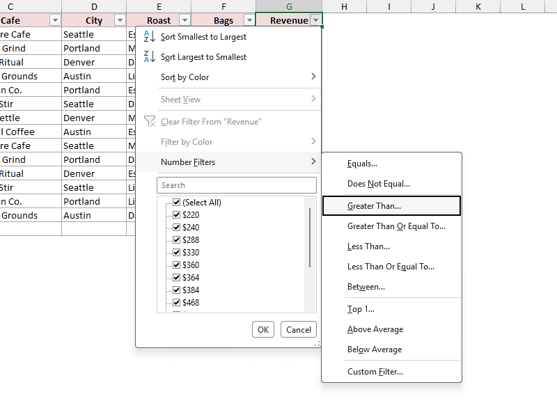
In the Custom Autofilter dialog box, type 500 and click OK.

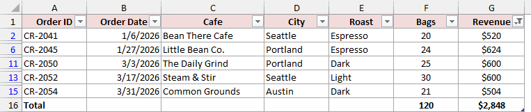
The Table now shows the five orders above $500, for a total of $2,848.

Text works the same way. On the Cafe filter, go to Text Filters > Contains and type Bean.

That keeps Bean There Cafe and Little Bean Co., which leaves four orders and $1,868.

A PivotTable has the same kind of condition filters on its row labels.

Here I’ve opened the Roast filter and used Value Filters > Greater Than to keep roasts with more than $1,500 in revenue.

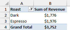
Only Dark ($1,776) and Espresso ($1,976) are left, and a slicer has no way to do that.

You don’t have to choose one or the other, though. A slicer and a condition filter work together when they’re on different columns.

Below, the City slicer is set to Seattle, and the Revenue column is filtered to greater than 500. Only two orders are left, for $1,120.

Also notice that Denver is greyed out in the slicer. None of the Denver orders are above $500, so the slicer dims it to show there’s nothing to see there.

Note: In a PivotTable, a slicer and a condition filter on the SAME field replace each other by default. To keep both, right-click the PivotTable, choose PivotTable Options, and check Allow multiple filters per field on the Totals & Filters tab.

Controlling Several PivotTables at Once

A Report Filter belongs to one PivotTable. If you have two PivotTables and want both to show Seattle, you have to set each filter separately.

A slicer can drive several PivotTables at once. Below, one City slicer controls both Revenue by Roast and Bags by Cafe, so clicking Seattle filters both.

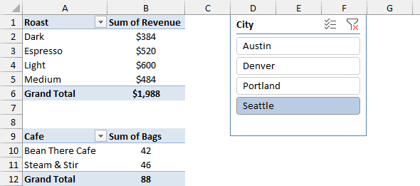
To connect a slicer to another PivotTable, select the slicer, go to the Slicer tab, and click Report Connections. Then check each PivotTable it should control.

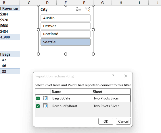
This only works when the PivotTables use the same data source. I’ve covered the full setup in my guide on how to connect a slicer to multiple PivotTables.

Space on the Sheet

A filter drop-down takes up no room at all. It lives inside the header cell.

A slicer is an object that sits on top of the cells, and each one covers a block of the sheet. With three or four slicers, you’re planning your layout around them.

Long lists make this worse.

A slicer with 50 cafe names needs a scroll bar, while the drop-down handles it easily and has a search box to find a name. A slicer has no search box.

Using Them on a Protected Sheet

Both tools can keep working after you protect a sheet, but you need to allow them in the Protect Sheet dialog box (Review > Protect Sheet).

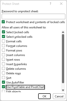
Check Use AutoFilter for a Table’s filter drop-downs and Table slicers. Check Use PivotTable and PivotChart for PivotTable filters and PivotTable slicers. You don’t need Edit objects.

Slicers need one more step. Excel locks every slicer by default, so a locked slicer stops working once the sheet is protected.

Before protecting the sheet, right-click the slicer, choose Size and Properties, and uncheck Locked under Properties.

Also make sure the Table’s filter arrows are showing before you protect the sheet, because you can’t turn them on afterwards.

Excel Versions, Mac, and Excel for the Web

Filter drop-downs work in every version of Excel, on every platform. Slicers came later and still have a few gaps:

• Slicers for PivotTables need Excel 2010 or later on Windows.
• Slicers for Tables need Excel 2013 or later on Windows.
• On a Mac, slicers need Excel 2016 or later. Current Mac versions support slicers for both Tables and PivotTables.
• In Excel for the web, you can click any slicer and insert a new one for a PivotTable. You can’t insert a slicer for a Table there, so add it in the desktop app first.
• The Excel apps for iPhone, iPad, and Android don’t support slicers.

In Excel for the web, the Report Connections option lives in a different place. Select the slicer, go to Slicer Settings, and use the PivotTable Connections section.

If people will open your file on a phone, a filter drop-down is the safer choice.

Report Filters vs Slicers

For PivotTables, the real comparison is between the Report Filter and the slicer. You’ve seen most of the differences already:

• A slicer can filter by any field. A Report Filter only works for a field in the Filters area.
• A slicer shows every selected item. A Report Filter shows (Multiple Items) once you pick more than one.
• A slicer can control several PivotTables. A Report Filter controls one.

The Report Filter has one trick of its own, called Show Report Filter Pages.

Select the PivotTable, go to PivotTable Analyze > Options (the small drop-down arrow) > Show Report Filter Pages, pick City, and click OK.

Excel creates one new sheet per city, named Austin, Denver, Portland, and Seattle. Each has a copy of the PivotTable filtered to that city, which is something a slicer can’t do.

When to Use a Slicer and When to Use a Filter

Here’s how I decide.

Use a slicer when:

• Other people will use the report and need to see what’s filtered.
• You’re building a dashboard where one click should update several PivotTables.
• The field has a short list of items, such as regions, cities, or product lines.

Use a filter drop-down when:

• You need a condition, such as greater than, between, contains, or top 10.
• The list is long and you need to search it.
• You just want a quick look at the data and don’t want an object on the sheet.
• The file will be opened on a phone or tablet.

And you can use both. A slicer for the main filter plus a condition filter on another column is a handy combination.

Additional Notes About Slicers and Filters in Excel

• Both tools hide rows, so SUM still adds the hidden ones. Use SUBTOTAL with 109 or a Table’s Total Row if the total should follow the filter.
• For dates, the filter drop-down groups dates by year, month, and day and has Date Filters like This Month. A slicer lists every date as its own button. For PivotTables, a Timeline is the slicer-style option for dates.
• Deleting a slicer doesn’t remove its filter. Clear the slicer first, then delete it.
• The example file has the Table with a City slicer, a PivotTable with a Report Filter, and two PivotTables sharing one slicer, so you can try both tools side by side.

Frequently Asked Questions

Can I use a slicer without a Table or PivotTable?

No. A slicer needs an Excel Table or a PivotTable.

For a normal range, select a cell in it and press Ctrl + T to make it a Table, then insert the slicer.

Can a slicer filter by greater than or a date range?

A slicer can’t filter by a condition like greater than. Use the filter drop-down for that. For a date range in a PivotTable, use a Timeline instead of a slicer.

Can one slicer control a Table and a PivotTable?

No. A slicer for a Table filters only that Table. A PivotTable slicer can connect to other PivotTables, but only ones built from the same data source.

Does a slicer replace the filter on a Table?

No, they share it. Clicking a slicer button sets the filter on that column, and the column’s drop-down shows the same selection.

Conclusion

In this article, I showed you the same filter done with a drop-down and with a slicer, first on a Table and then on a PivotTable.

I also compared the two on conditions, several PivotTables, protected sheets, and Excel for the web, and covered when to pick each one.

I hope you found this article helpful.

Other Excel articles you may also like:

• How to Filter Multiple Columns in Excel?
• How to Count Filtered Rows in Excel?
• Excel Filter Not Working – How to Fix?
• How to Filter by Color in Excel?
• How to Lock a Pivot Table in Excel
• Pivot Table vs Pivot Chart in Excel
• How to Refresh Pivot Table in Excel? (Shortcut + VBA)
• Display Selected Slicer Items in a Cell
• Slicer Not Working or Greyed Out