
A slicer in Excel lists its buttons in alphabetical order by default. That’s fine for product names, but not for things that have a natural order.
Shifts should run Morning, Afternoon, Evening, not Afternoon, Evening, Morning. And months that show up as April, February, January make a report hard to read.
The catch is that you can’t drag slicer buttons into place. The order comes from the slicer’s sort settings, a custom list, or the data behind it.
In this article, I’ll show you how to sort slicer items with a custom list, fix months that are out of order, and sort by another column.
Method #1: Using the Sort Commands on the Slicer
If all you need is A to Z or Z to A, you can sort a slicer with two clicks.
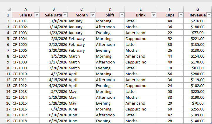
Below I have the sales data for a small coffee shop. Each sale has a date, the month, the shift, the drink, the cups sold, and the revenue.
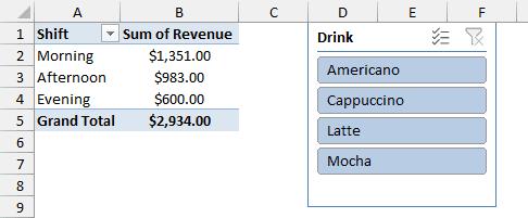
I’ve made a PivotTable from this data that shows revenue by shift, and added a Drink slicer next to it. The buttons are in A to Z order.
Now I want the drinks listed from Z to A instead.
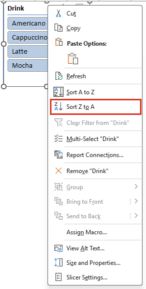
To do this, right-click the slicer and choose Sort Z to A.
The Drink slicer now lists Mocha, Latte, Cappuccino, and Americano.
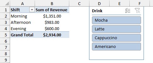
This only changes the slicer. The PivotTable keeps its own sort order.
Method #2: Using a Custom List (Recommended)
When your items have an order that isn’t alphabetical, a custom list is the way to go. You tell Excel the order once, and the slicer follows it.
I’m using the same PivotTable of revenue by shift. This time it has a Shift slicer.
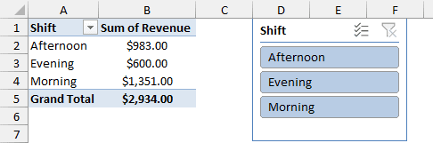
The slicer shows Afternoon, Evening, and Morning. I want Morning, Afternoon, and Evening, the order the shifts happen in the day.
Here are the steps to create the custom list:
- Click File and then Options.
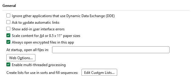
- In Excel Options, click Advanced, scroll down to the General section, and click Edit Custom Lists.
- In the Custom Lists dialog box, type Morning, Afternoon, and Evening in the List entries box, one per line. Click Add, then click OK twice.
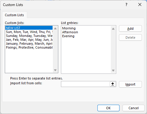
If your items are already typed in cells, click in the Import list from cells box, select those cells, and click Import instead.
The slicer doesn’t change yet. Excel applies the new list the next time the PivotTable refreshes.
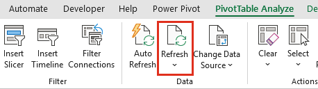
- Select any cell in the PivotTable, go to the PivotTable Analyze tab, and click Refresh.
The Shift slicer now shows Morning, Afternoon, and Evening. You don’t need to delete the slicer and insert it again.
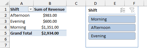
This works because the Use Custom Lists when sorting box in Slicer Settings is checked by default.
If your slicer ignores the list, right-click the slicer, choose Slicer Settings, and make sure that box is checked.
Note: The custom list is saved in Excel on your computer, not in the workbook. On a computer without the list, the file keeps your order until the PivotTable refreshes. Then the slicer goes back to A to Z.
Method #3: Using the Built-In Month Lists
Months that sort as April, February, January are one of the most common slicer problems. Excel already has a custom list for months, so you don’t need to make one.
Below is the same PivotTable of revenue by shift, now with a Month slicer. The slicer lists the months alphabetically.
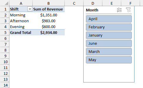
Excel comes with four built-in lists: short and long day names (Sun, Sunday) and short and long month names (Jan, January).
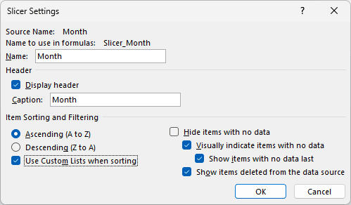
A slicer uses them only when Use Custom Lists when sorting is checked, which it is by default.
So if your months are out of order, the box has been unchecked, the names don’t match the list, or the PivotTable uses the Data Model (see Method #5).
Here are the steps to put the months in calendar order:
- Right-click the Month slicer and choose Slicer Settings.
- Check Use Custom Lists when sorting and click OK.
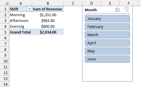
The slicer now runs from January to June.
Note: The month names must match the built-in list exactly. January or Jan works, but Sept doesn’t, because the list uses Sep. An item that isn’t in any list drops to the end of the slicer.
Method #4: Using Real Dates Instead of Text Months
The built-in lists sort by month name, not by year.
If your months are text labels like Nov 2025 and Jan 2026, the slicer sorts them alphabetically, and no list can fix that.
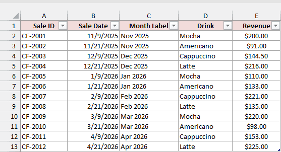
Below I have 12 sales from November 2025 to April 2026. The Month Label column holds text, like Nov 2025.
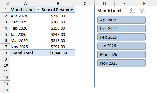
When I make a slicer from Month Label, it starts with Apr 2026 and ends with Nov 2025.
The fix is to give the slicer real dates. A date sorts by its value, so the months stay in timeline order even across a new year.
I’ve added a Month Start column that returns the first day of each sale’s month. Here is the formula:
=EOMONTH(B2,-1)+1
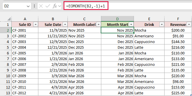
The EOMONTH function with -1 returns the last day of the month before the sale date.
Adding 1 moves it to the first day of the sale’s month, so every November 2025 sale gets November 1, 2025.
Because the data is an Excel Table, Excel fills the formula down the column for you.
I’ve formatted the column with the custom number format mmm yyyy, so it shows Nov 2025 instead of a full date.
Now refresh the PivotTable, then insert a slicer for Month Start (PivotTable Analyze > Insert Slicer). The slicer runs from Nov 2025 to Apr 2026.
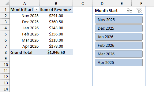
Since each month has a single date, the slicer shows one button per month, not one per day.
Method #5: Using Sort by Column in the Data Model
If your PivotTable was made with Add this data to the Data Model checked, custom lists don’t work.
A Data Model slicer doesn’t have the Use Custom Lists when sorting option at all.
Here’s the same coffee shop data in a Data Model PivotTable, with a Month slicer. The months are alphabetical.
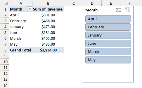
Instead of a list, the Data Model sorts a column by another column. So first, you need a column that holds the right order.
I’ve added a Month No column to the Table with this formula:
=MONTH(B2)
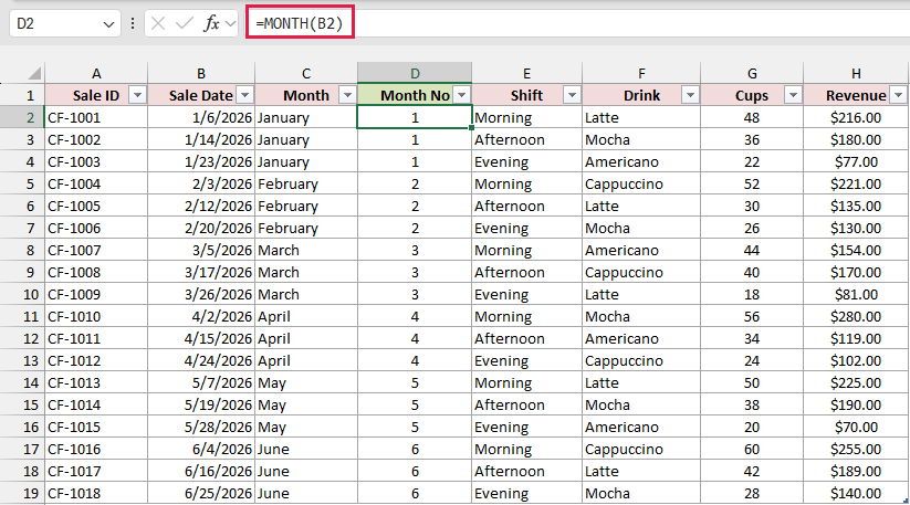
The MONTH function returns the month number of the sale date, so January is 1 and June is 6. Refresh the PivotTable so the new column reaches the Data Model.
Here are the steps to sort Month by Month No:
- Go to the Power Pivot tab and click Manage. If you don’t see the tab, go to File > Options > Add-ins, choose COM Add-ins in the Manage box, click Go, and check Microsoft Power Pivot for Excel.

- In the Power Pivot window, click the Month column header. On the Home tab, click Sort by Column.
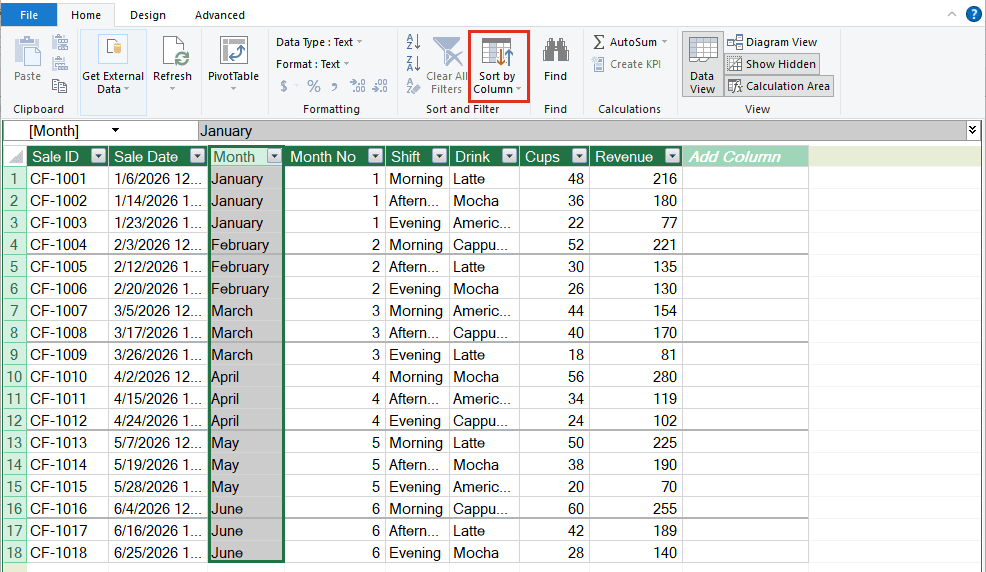
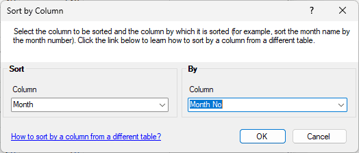
- In the Sort by Column dialog box, check that Month is selected under Sort. Under By, choose Month No and click OK.
- Close the Power Pivot window and refresh the PivotTable.
The Month slicer now lists January to June, and so do the PivotTable rows.
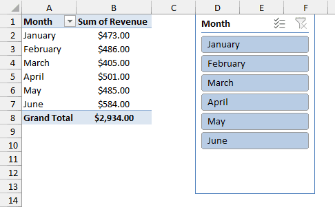
Note: Leave the slicer’s sort on Data source order, which is the default for Data Model slicers. If you switch it to Ascending or Descending, Excel sorts the month names alphabetically again.
This is also how you sort a slicer by another column. Any column of numbers can set the order, like a priority rank or a size code.
Additional Notes About Custom Sorting Slicer Items in Excel
- Months can jump to the bottom when you filter. By default, when another slicer leaves a month with no data, Excel moves that month to the end. To stop this, uncheck Show items with no data last in Slicer Settings.
- New items land at the end. If your data gets a value that isn’t in your custom list, the slicer puts it after the listed items, in A to Z order. Add it to the list to fix it.
- The PivotTable has its own sort. Sorting the slicer doesn’t move the PivotTable rows. To match them, sort the PivotTable too, or reorder the rows in the pivot table by hand.
- Descending reverses a custom list. With a custom list in use, Descending gives you Evening, Afternoon, Morning.
- These steps are for Excel on Windows. The menus differ on a Mac, and Power Pivot (needed for Method #5) isn’t available in Excel for Mac.
Frequently Asked Questions
A few more questions that come up when you sort slicer items.
Can I drag slicer buttons into a different order?
No. Slicer buttons can’t be moved by hand. The order always comes from the sort setting, a custom list, or a sort-by column in the Data Model.
Do I need to recreate a slicer after adding a custom list?
No. Refresh the PivotTable and the slicer re-sorts. A slicer you insert after creating the list uses it straight away.
Can I sort slicer items by sales or another value?
No. Slicer Settings sorts by the item names only, so it can’t order buttons by their sales.
Why is Use Custom Lists when sorting missing from Slicer Settings?
Your PivotTable uses the Data Model. Data Model slicers follow the column’s sort order instead, so use Sort by Column (Method #5).
Conclusion
In this article, I showed you five ways to custom sort slicer items, including custom lists, real dates, and Sort by Column in the Data Model.
For most slicers, a custom list plus a PivotTable refresh is all you need.
I hope you found this article helpful.
Other Excel articles you may also like:
- Connect Slicer to Multiple Pivot Tables (Step-by-Step)
- How to Use a Pivot Table Timeline in Excel (Step-by-Step)
- Slicer Not Working or Greyed Out in Excel? (20 Easy Fixes)
- How to Show Slicer Selection in a Cell in Excel (4 Easy Ways)
- Slicers vs Filters in Excel (Differences and When to Use Each)
- Create Interactive Dashboard in Excel (Free Download)
- How to Group by Months in Excel Pivot Table?
- How to Sort Alphabetically in Excel (6 Easy Ways)
- Change Slicer Style and Colors
- Search Slicer Items in Excel
