How to Add a Search Box to a Slicer in Excel (3 Easy Ways)

A slicer is great when it has five buttons. When it has 36, you end up scrolling up and down the list, hunting for the one item you want.

Excel slicers don’t have a search box. There’s no setting for it in Slicer Settings or on the Slicer tab, in any version of Excel.

What you can do is borrow a search box from somewhere else. A PivotTable’s filter drop-down has one, and so does the filter arrow in an Excel Table.

In this article, I’ll show you three ways to search a slicer: a small PivotTable connected to it, the search box in a Table’s filter, and a FILTER formula.

Table of Contents

Method #1: Using a Second PivotTable as a Search Box

This is the method I’d use for most dashboards.

You add a tiny second PivotTable that only has a filter drop-down, connect it to the same slicer, and park it right above the slicer.

When you search in that drop-down, the slicer picks up the same items.

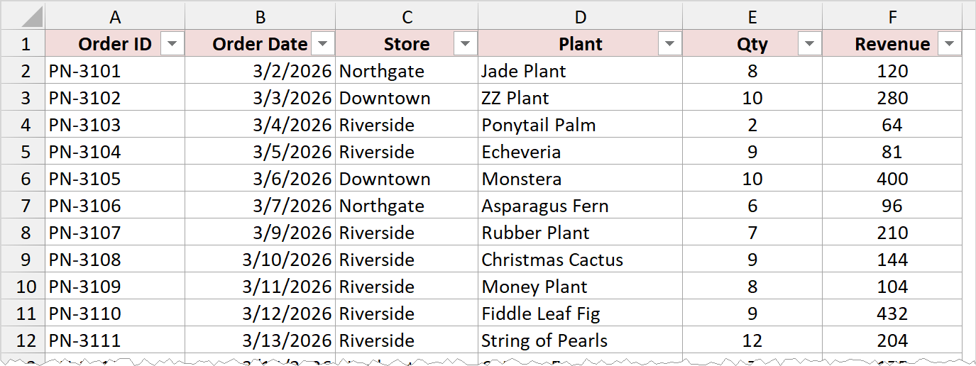
Below I have a dataset of 40 orders from a plant nursery. Each order has an order ID, a date, a store, the plant sold, the quantity, and the revenue.

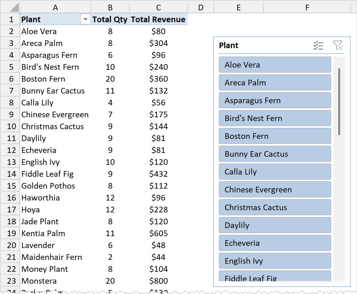
Plant nursery Table of 40 orders with order ID, date, store, plant, quantity, and revenue

I’ve made a PivotTable from this data that shows the quantity and revenue for each plant, with a Plant slicer next to it.

There are 36 plants, so the slicer only shows about a dozen at a time.

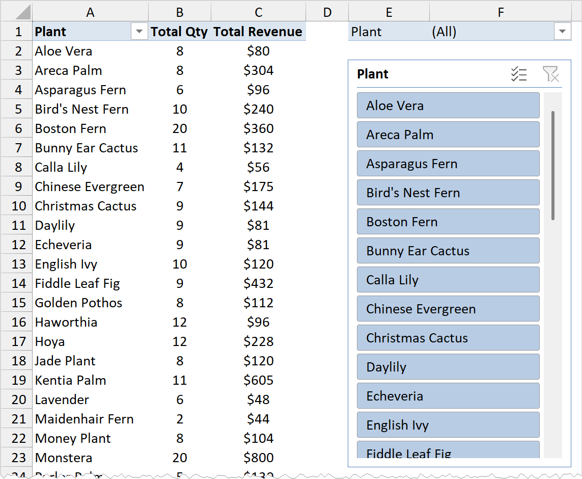
I’ve left two empty rows above the slicer, which is where the search box will go.

PlantSummary PivotTable with a 36-item Plant slicer that needs scrolling, two empty rows above it

Here are the steps to add a search box to this slicer:

Select any cell in the PivotTable and press Ctrl + C. Then select cell E1, right above the slicer, and press Ctrl + V.

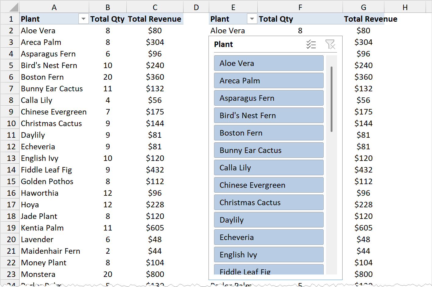
A copy of the PivotTable pasted at E1, mostly hidden behind the slicer

Excel pastes a full copy of the PivotTable, and most of it sits behind the slicer. That’s fine, because you’re about to cut it down to one row.

The copy also shares the original PivotTable’s data, so the slicer is already connected to it.

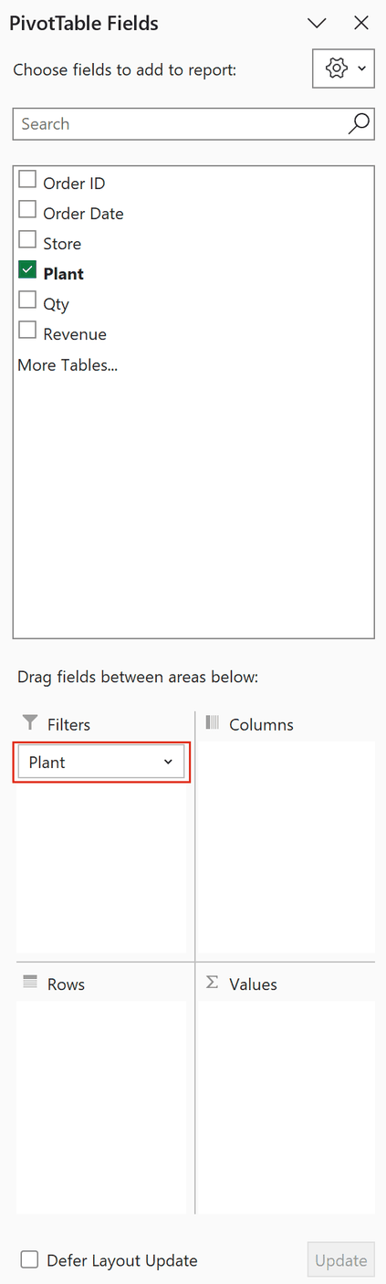
With a cell in the copy still selected, go to the PivotTable Fields pane. Uncheck Total Qty and Total Revenue, then drag Plant from the Rows area to the Filters area.

PivotTable Fields pane with Plant in the Filters area and nothing in Rows or Values

The copy shrinks to a single row in E1:F1. It shows the field name, Plant, and its current filter, (All), with a drop-down arrow.

The copy reduced to one row in E1:F1, Plant (All), sitting above the slicer

Right-click any cell in the new PivotTable and click PivotTable Options. On the Layout & Format tab, make sure Autofit column widths on update is unchecked, then click OK.

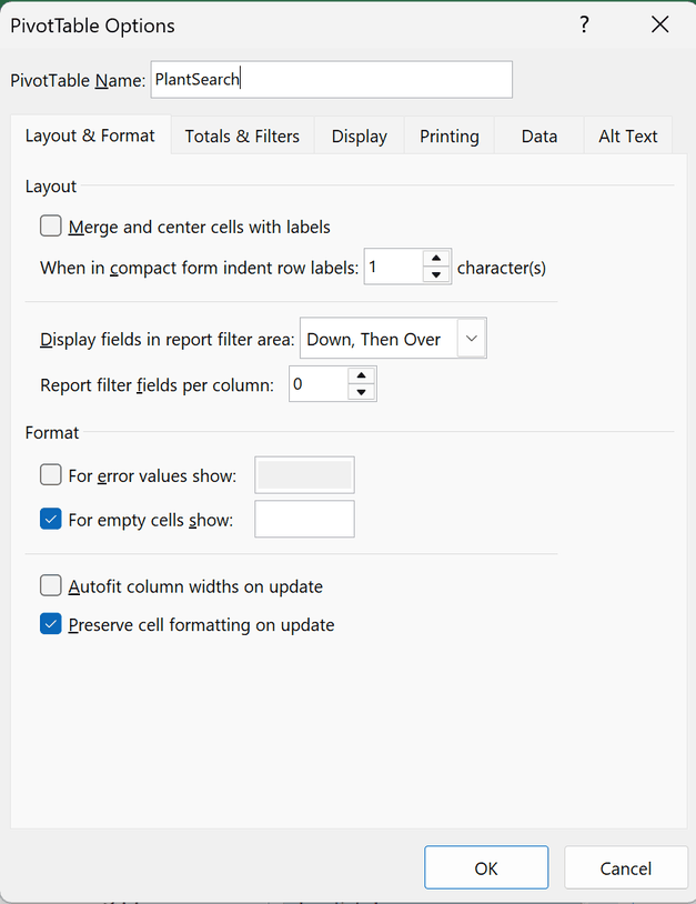
PivotTable Options, Layout & Format tab, Autofit column widths on update unchecked

If you leave Autofit on, Excel resizes columns E and F every time the filter changes. The search box then jumps around and no longer lines up with the slicer.

Right-click the slicer and click Report Connections. Make sure both PivotTables are checked, then click OK.

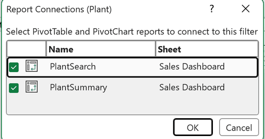
Report Connections dialog with both PivotTables checked

Now you can search the slicer.

Click the drop-down arrow in cell F1 and check Select Multiple Items at the bottom of the list. Then type fern in the Search box and click OK.

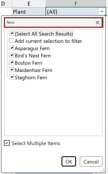
Report filter drop-down searching fern with the five ferns checked

The slicer now highlights the five ferns, and the PivotTable shows only those five plants. The Grand Total drops from $6,561 to $950.

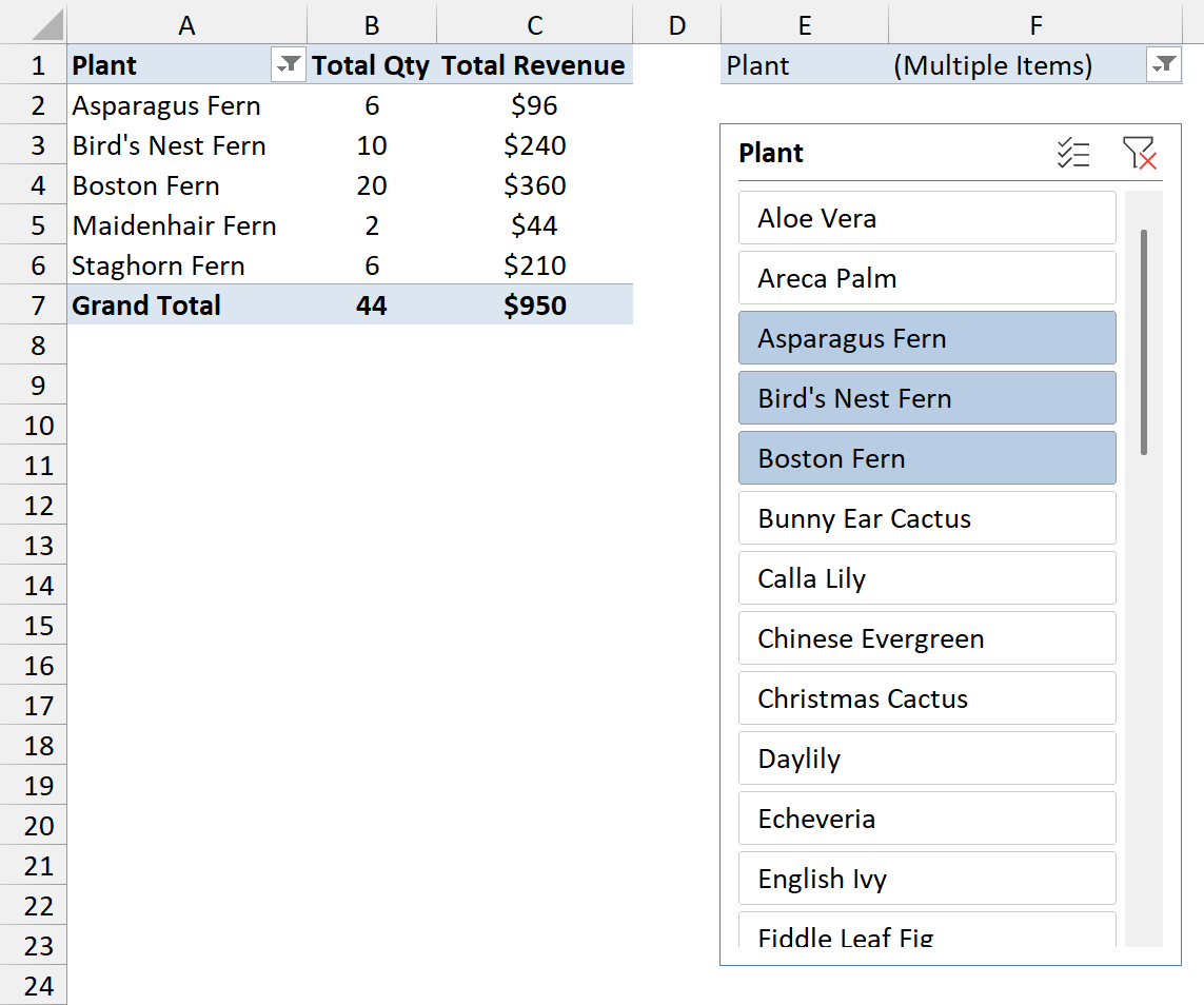
Slicer highlights the ferns and the PivotTable shows five fern plants totaling $950; F1 shows (Multiple Items)

You may need to scroll the slicer to see all five highlighted buttons, because the non-fern plants stay in the list, just not selected.

Cell F1 now says (Multiple Items), which tells you a search filter is active.

To go back to all the plants, click the Clear Filter button in the slicer’s top-right corner.

Note: Check Select Multiple Items before you search, so every matching plant gets selected when you click OK.

Method #2: Using the Table Filter Search

If your slicer is connected to an Excel Table instead of a PivotTable, you don’t need a second object.

The Table’s own filter arrows already have a search box, and they filter the same rows as the slicer.

Below I have the same 40 plant orders, this time as an Excel Table with a Plant slicer beside it.

Plant orders as an Excel Table with a Plant slicer beside it

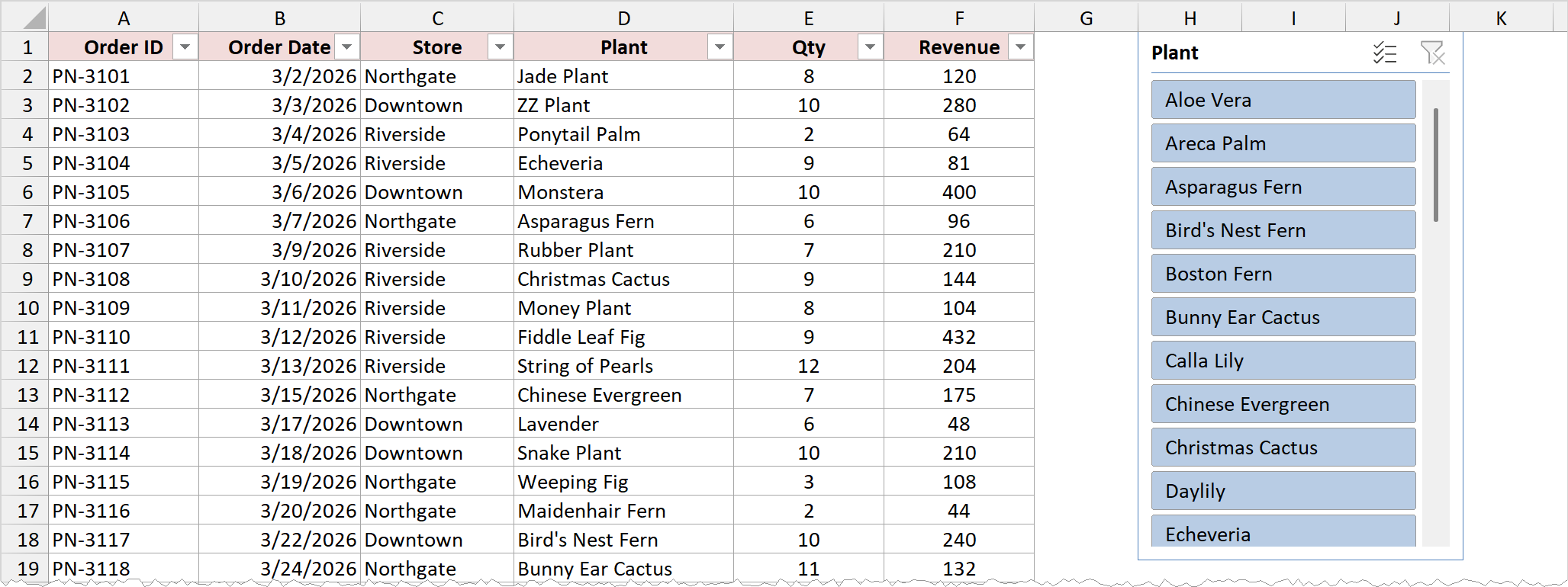
Here are the steps to search the Plant column:

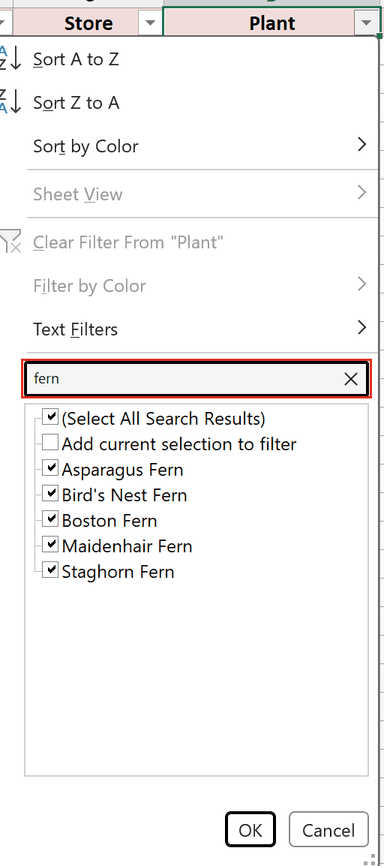
Click the filter arrow in the Plant header. Type fern in the Search box and click OK.

The Table now shows only the six fern orders, and the slicer highlights the five ferns. Boston Fern shows up twice because it was sold twice.

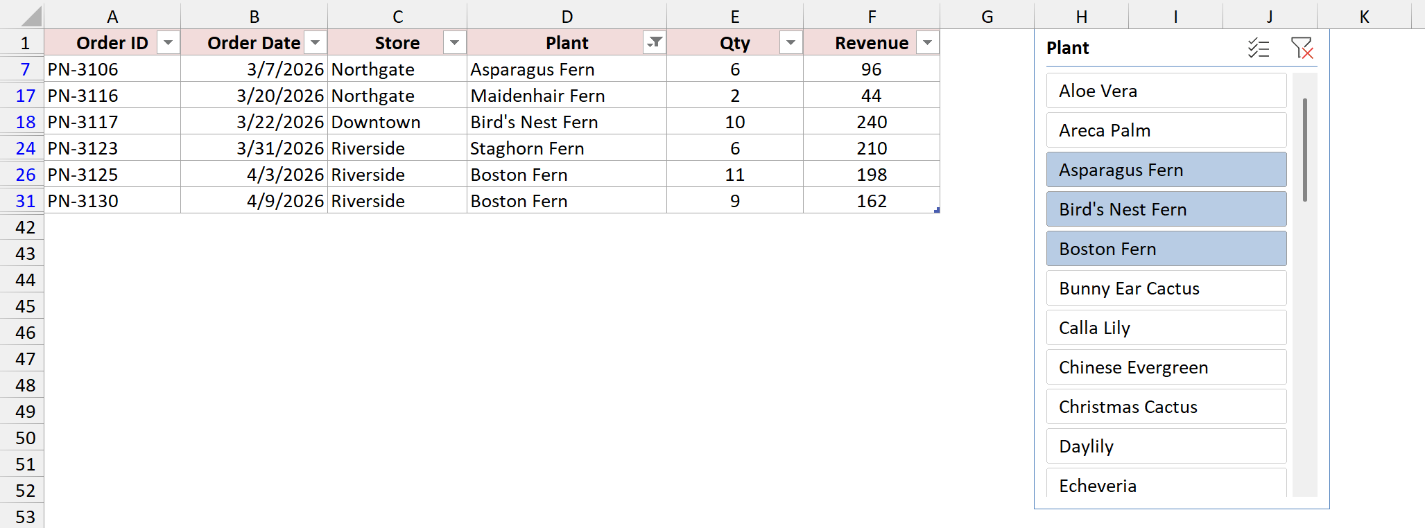
To bring all the rows back, click the filter arrow in the Plant header again and choose Clear Filter From “Plant”.

Note: A Table slicer needs Excel 2013 or later. The search box in the filter drop-down has been there since Excel 2010.

Method #3: Using the FILTER and SEARCH Functions

The first two methods borrow a search box from a drop-down. If you’d rather type into a cell and filter as you type, a formula can do that.

This one doesn’t control the slicer. It builds a separate, searchable report from the same data, which works well as a lookup sheet next to your dashboard.

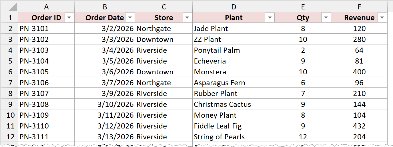
Below I have the same 40 plant orders in an Excel Table named PlantSales.

Plant nursery Table of 40 orders named PlantSales

On a new sheet, I’ve typed Search Plant in cell A1 and the search term fern in cell B1. Row 3 has the same headers as the Table.

Here is the formula in cell A4:

=FILTER(PlantSales,ISNUMBER(SEARCH(B1,PlantSales[Plant])),"No matches")

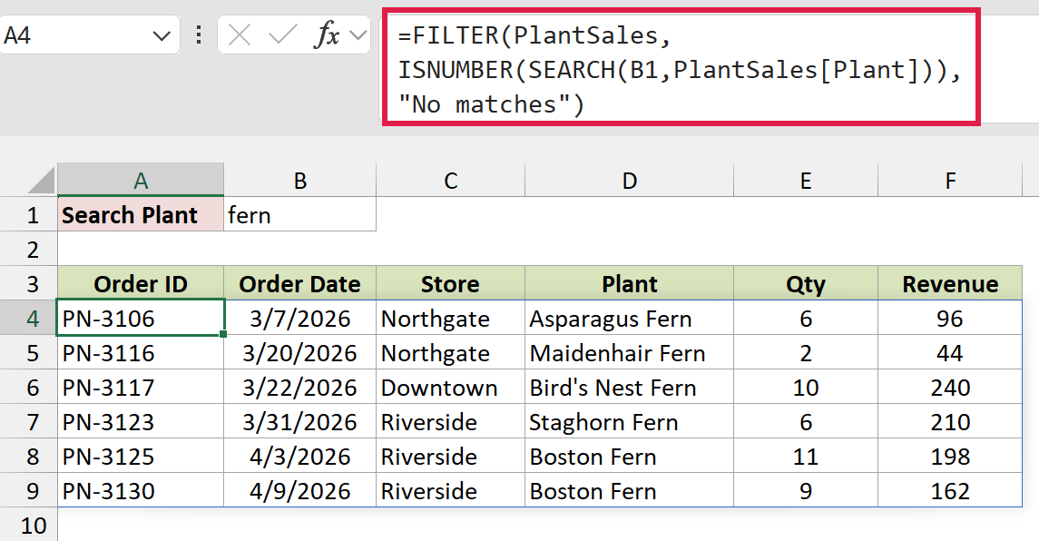
FILTER and SEARCH formula in A4 returning the six fern orders for the search term in B1

The formula returns the six fern orders, and the results spill down the sheet automatically.

FILTER returns dates as plain numbers, so I’ve formatted column B as a date.

How does this formula work?

SEARCH(B1,PlantSales[Plant]) looks for the text in B1 inside every plant name. It returns the position where the text starts, or a #VALUE! error when the text isn’t there.

ISNUMBER turns those results into TRUE for a match and FALSE for everything else.

FILTER then returns every row of the Table where the result is TRUE. If nothing matches, it returns “No matches” instead of an error.

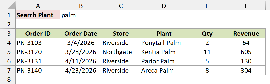
Now type palm in cell B1. The results change right away to the four palm orders.

Search term changed to palm, formula returns the four palm orders

Note: FILTER is available in Excel 2021, Excel 2024, and Microsoft 365. It doesn’t work in Excel 2019 or earlier.

Additional Notes About Adding a Search Box to a Slicer in Excel

All three searches match text anywhere in the name, not only at the start. Searching lily returns Peace Lily, Calla Lily, Tiger Lily, and Daylily.
None of them care about upper or lower case. Fern, FERN, and fern all return the same plants.
When you add new rows to the data, refresh the PivotTables with Data > Refresh All. New plants then show up in both the slicer and the search drop-down, because the two PivotTables share the same data.

Frequently Asked Questions

Here are a few questions people often ask about slicer search boxes.

Does Excel have a built-in search box for slicers?

No. Excel slicers have no search option in any version. Power BI slicers have one, so if you’ve seen a searchable slicer, it was probably in a Power BI report.

Does the search box work if my slicer controls several PivotTables?

Yes. The search PivotTable is one more connection on the slicer. When a search changes the slicer, every PivotTable connected to it filters too.

Why does the search box show (Multiple Items)?

That’s how a PivotTable filter tells you more than one item is selected.

It appears after any search that matches more than one plant, and it goes back to (All) when you clear the slicer.

Conclusion

Excel doesn’t give slicers a search box, but a small PivotTable parked above the slicer comes close. For a PivotTable dashboard, that’s the method I’d pick.

If your slicer sits on an Excel Table, search the Table’s own filter drop-down.

And if you want results as you type, the FILTER and SEARCH formula gives you a live search report.

I hope you found this article helpful.

Other Excel articles you may also like: