How to Filter Horizontally in Excel (Filter Across Columns)

Excel’s Filter button only works one way. It hides rows, so it can’t help when your data runs sideways, with each record in its own column.

You see this layout a lot in comparison sheets and monthly reports, where the field names sit down column A and every column to the right is one item.

There’s no setting that flips the filter to work left to right. But you can still show only the columns you want.

You can pull the matching columns out with a formula, hide the columns that don’t match, or turn the data upright so the regular filter works.

In this article, I’ll show you four ways to filter horizontally, using the FILTER function, Go To Special, Paste Special with the regular filter, and Power Query.

Method #1: Using the FILTER Function

This is the method I recommend for most people. It’s one formula, and the result updates on its own when your data changes.

Below I have a dataset of apartment listings. Each listing sits in its own column, with its city, number of bedrooms, and monthly rent in the rows below.

I want to show only the listings in Austin.

I’ve typed the same row labels (Listing, City, Bedrooms, Monthly Rent) in A6:A9, so the result is easy to read. Here is the formula I entered in B6:

=FILTER(B1:K4,B2:K2="Austin")

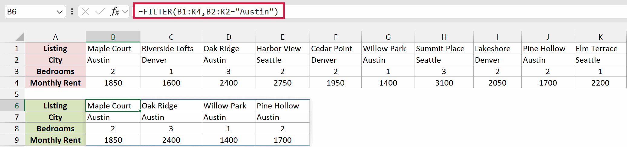
The result spills across and down automatically. You get the four Austin listings: Maple Court, Oak Ridge, Willow Park, and Pine Hollow.

How does this formula work?

The FILTER function keeps the parts of a range that meet a condition. Most people use it to keep rows, but it works on columns too.

The condition B2:K2=”Austin” checks each cell in the City row and returns a row of TRUE and FALSE values, one for each listing.

That row is as wide as B1:K4, so FILTER keeps every column where the check is TRUE and drops the rest.

You can also filter on more than one condition. This formula keeps the Austin listings with a rent of 2,000 or less:

=FILTER(B1:K4,(B2:K2="Austin")*(B4:K4<=2000))

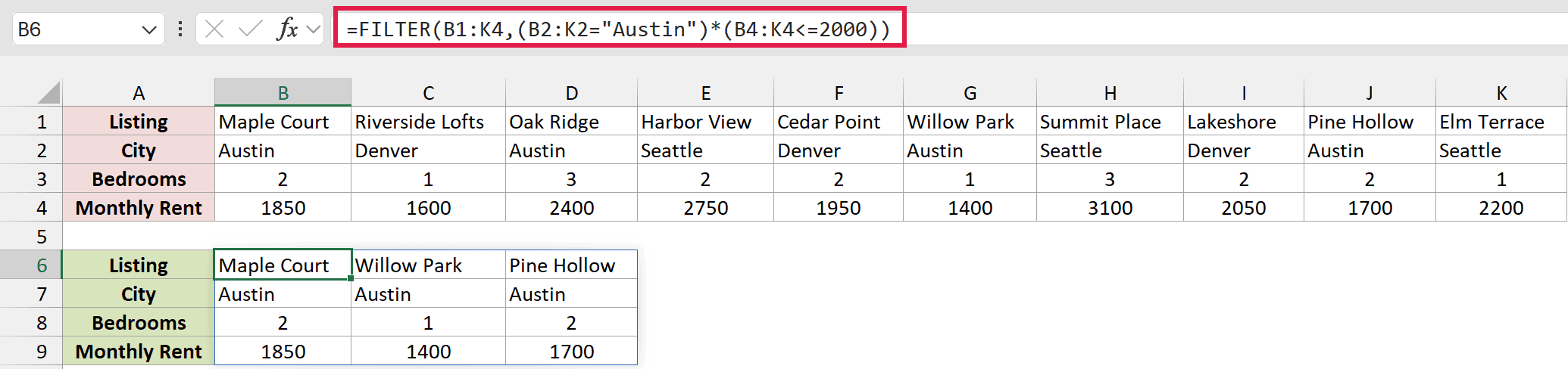
Oak Ridge drops out because its rent is 2,400. That leaves Maple Court, Willow Park, and Pine Hollow.

Multiplying the two checks works like AND, so a column is kept only when both are TRUE.

To keep columns that match either condition, add the checks with a plus sign instead.

For example, =FILTER(B1:K4,(B2:K2=”Austin”)+(B2:K2=”Denver”)) returns the seven listings in Austin or Denver.

Note: FILTER is available in Excel 365 and Excel 2021 or later. If you’re on an older version, use one of the other methods below.

Method #2: Using Go To Special (Row Differences)

If you’d rather hide the other columns right where they are, this one is for you. It works in every version of Excel, and you don’t need a formula.

Below I have the same apartment listings, with the city for each listing in row 2.

I want to hide every listing that isn’t in Austin.

This method uses a Go To Special option called Row differences.

It selects every cell in a row that’s different from the active cell, which is the white cell in your selection.

Here are the steps to hide the columns that don’t match:

1. Select B2:K2, starting from B2. B2 holds Austin, so it becomes the active cell and the value Excel compares against.

If the value you want isn’t in the first cell, press Tab to move the active cell to a cell that has it. The selection stays the same.

2. On the Home tab, click Find & Select, then Go To Special.

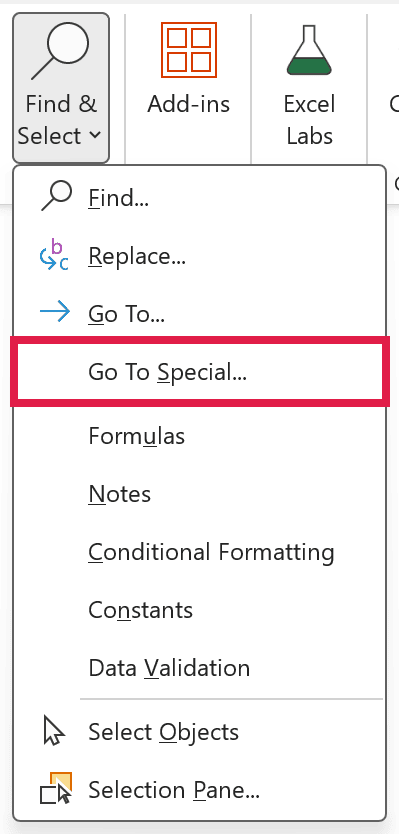
3. In the Go To Special dialog box, select Row differences and click OK.

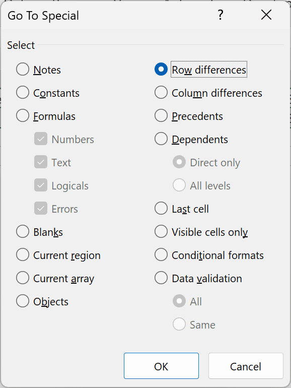
Excel now selects every cell in the City row that isn’t Austin. The check ignores case, so austin and AUSTIN count as a match too.

4. Press Ctrl + 0 to hide the columns of the selected cells. You can also go to Home, then Format, then Hide & Unhide, then Hide Columns.

Only the four Austin listings are left. Columns C, E, F, H, I, and K are hidden.

To bring them back, select the column headers from A to K, right-click, and choose Unhide.

Row differences only finds cells that are different from the active cell. So it works for “equal to” filters, but not for conditions like “rent under 2,000”.

Note: Hidden columns still get copied when you copy the range. To copy only the visible listings, select the range, press Alt + ; (or use Go To Special, then Visible cells only) to select the visible cells, then copy.

Method #3: Using Paste Special Transpose and Filter

Here’s another way to do this, using the regular Filter button. You convert the columns to rows so each listing gets its own row, then filter it the normal way.

Below I have the apartment listings again, laid out across columns A to K.

I want a copy of this data that I can filter by city.

Here are the steps to transpose the data and filter it:

1. Select A1:K4 and press Ctrl + C (Cmd + C on a Mac) to copy it.

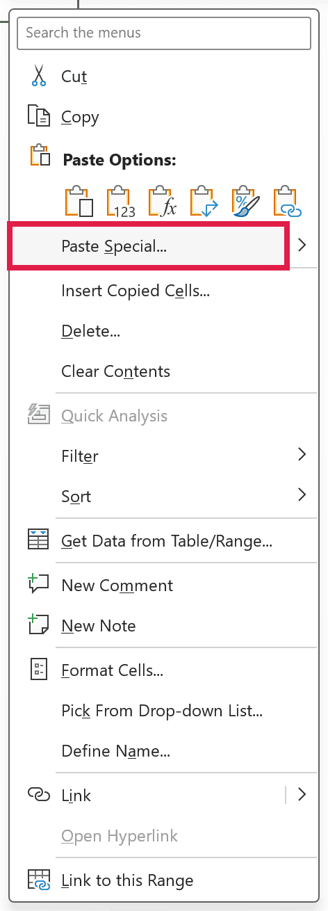
2. Right-click cell A6 and choose Paste Special.

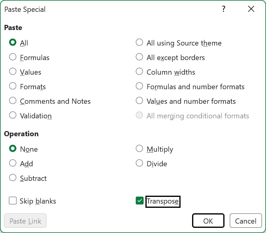
3. In the Paste Special dialog box, check Transpose and click OK.

Excel pastes the data upright in A6:D16. Listing, City, Bedrooms, and Monthly Rent are now the column headers, and each apartment has its own row.

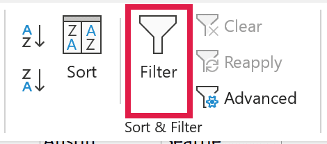
4. Select any cell in the new table, go to the Data tab, and click Filter.

5. Click the filter button in the City header. Uncheck Select All, then check Austin.

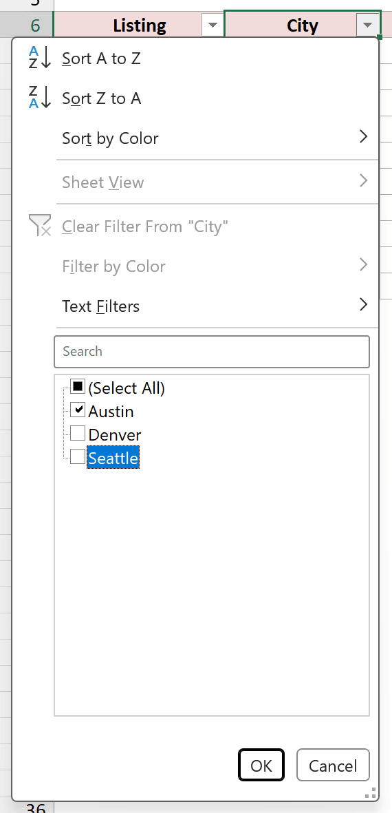
6. Click OK.

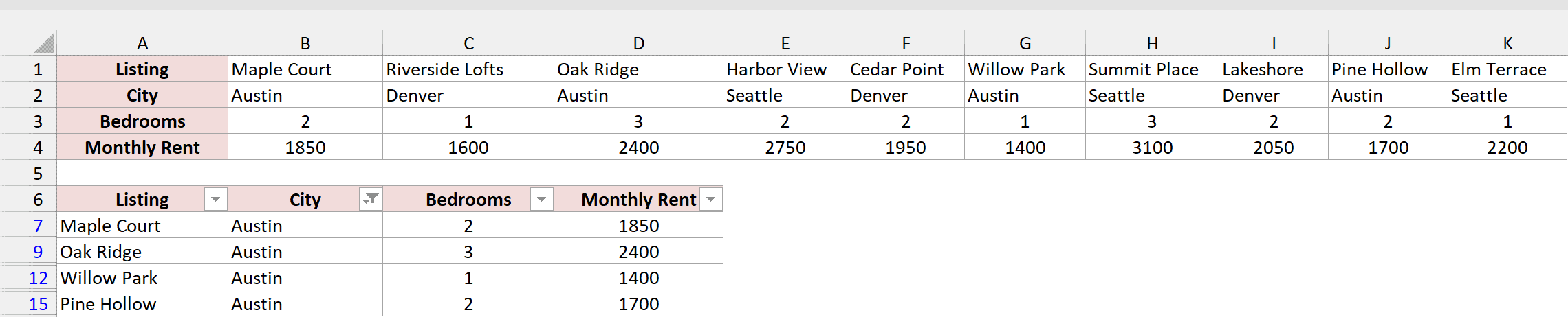
Only the four Austin listings are left in the table. You can now sort and filter them on any other column too, like keeping only the two-bedroom places.

Note: The transposed table is a copy, not a link. If you change the original data, you’ll need to copy and transpose it again.

Method #4: Using Power Query

If you get fresh data in the same sideways layout every week, Power Query can do the flip, the filter, and the flip back for you.

You set it up once and refresh it.

Below I have the apartment listings again in A1:K4, with the listing names in row 1.

I want a table that shows only the Austin listings and stays in the same sideways layout.

Here are the steps to filter the columns with Power Query:

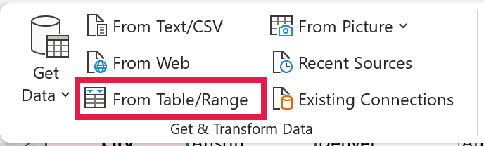
1. Select any cell in the data. Go to the Data tab and click From Table/Range.

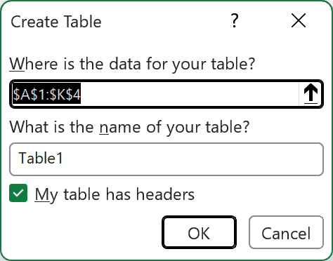
2. In the Create Table dialog box, make sure My table has headers is checked and click OK.

Excel turns the data into a table, with the listing names as its headers, and opens the Power Query Editor.

Power Query filters rows, so the first job is to turn the listings into rows. To do that, the listing names have to move out of the headers first.

3. On the Home tab, click the drop-down arrow next to Use First Row as Headers and choose Use Headers as First Row.

4. Go to the Transform tab and click Transpose.

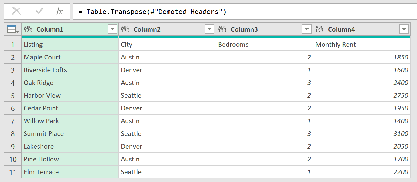
5. Click Use First Row as Headers.

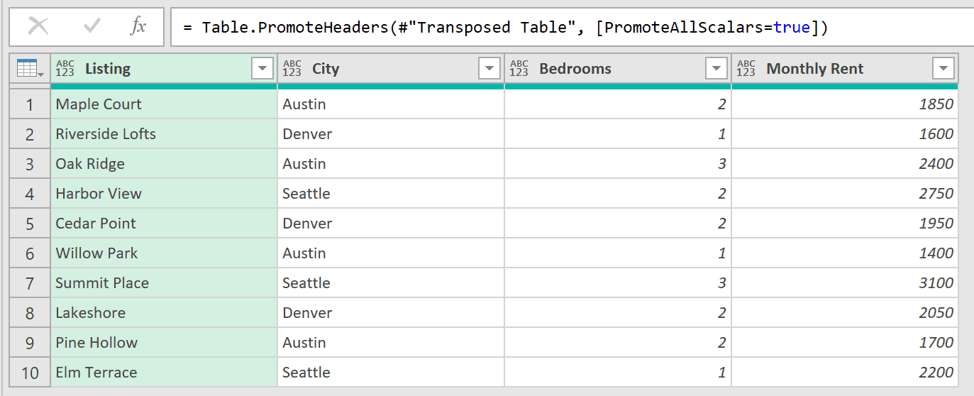
Each listing is now a row, under the headers Listing, City, Bedrooms, and Monthly Rent.

6. Click the filter arrow in the City header, uncheck everything except Austin, and click OK.

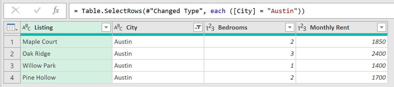
If you’re happy with the listings as rows, you can skip to step 8. The next step turns them back sideways.

7. Repeat steps 3 to 5: choose Use Headers as First Row, click Transpose, then click Use First Row as Headers.

8. On the Home tab, click Close & Load.

Power Query loads the result as a new table on a new sheet. It has the four Austin listings, laid out across the columns like the original.

Power Query may add a few Changed Type steps on its own as you go. That’s normal, and you can leave them.

Note: The loaded table doesn’t update by itself. When you add or change listings in the source table, go to the Data tab and click Refresh All.

Additional Notes About Filtering Horizontally in Excel

• Excel’s filter tools only work top to bottom. That includes the Filter button, slicers, and Advanced Filter. Sort can go left to right through its Options button, but Filter has no such option.
• Only the FILTER formula updates on its own. Go To Special and the transposed copy are one-time results. Power Query updates when you click Refresh All.
• For hiding that happens automatically, you’ll need a macro. A short VBA macro can hide columns based on a cell value every time the value changes.
• If you control the layout, put each record in a row. Excel’s sorting, filtering, PivotTables, and slicers are all built for that shape, so you won’t need any of these workarounds.

Frequently Asked Questions

Here are answers to a few questions people often ask about filtering horizontally in Excel.

Can I add filter buttons to a row in Excel?

No. Filter buttons always go on a header row and filter the rows below it.

To use filter buttons on sideways data, transpose it first (Method #3), or use the FILTER function instead.

Does the FILTER function work horizontally in Excel 2019?

No. FILTER needs Excel 365 or Excel 2021 or later, so Excel 2019 shows a #NAME? error.

In older versions, use Go To Special, the transpose method, or Power Query, which is built into Excel 2016 and later.

Why does my FILTER formula return #CALC!?

FILTER returns #CALC! when no column matches your condition, like a city that isn’t in the data.

Add a third argument to show a message instead: =FILTER(B1:K4,B2:K2=”Boston”,”No match”).

How do I show the filtered result as a vertical list?

Wrap the formula in the TRANSPOSE function: =TRANSPOSE(FILTER(B1:K4,B2:K2=”Austin”)).

Each Austin listing then gets its own row, with Listing, City, Bedrooms, and Monthly Rent across the columns.

Conclusion

In this article, I showed you four ways to filter horizontally in Excel, using the FILTER function, Go To Special, Paste Special with the regular filter, and Power Query.

If you have Excel 365 or Excel 2021, the FILTER formula is the one to reach for. It’s quick to set up and keeps itself up to date.

I hope you found this article helpful.

Other Excel articles you may also like:

• How to Filter Multiple Columns in Excel?
• CHOOSECOLS Function in Excel
• How to Hide Rows based on Cell Value in Excel?
• How to Use Custom AutoFilter in Excel (AND/OR Conditions and Wildcards)
• Slicers vs Filters in Excel (Differences and When to Use Each)
• Excel Filter Not Working: How to Fix?
• How to Paste into Filtered Column Skipping the Hidden Cells?
• Row vs Column in Excel – What’s the Difference?