How to Organize Excel Tabs Under a Master Sheet

If your Excel workbook has grown to a dozen tabs, you’ve probably wished you could tuck some of them under one main tab, the way folders work on your computer.

Excel can’t do that. There are no nested or child tabs, so every sheet sits side by side on the same flat strip at the bottom of the window.

What you can do is build a master sheet that works like a front page. It lists the other tabs, takes you to any of them in one click, and can even pull their totals together.

In this article, I’ll show you six ways to organize your tabs, including a clickable index with Insert Link or the HYPERLINK function, tab colors, hidden helper sheets, a 3D reference summary, and a macro that rebuilds the index.

Method #1: Using the Insert Link Option

This is the method I’d recommend for most workbooks. You turn each sheet name on your master sheet into a link, so clicking it opens that tab. You don’t need any formulas or macros for this one.

Below I have the Master sheet of a small bakery workbook. Column A lists the other tabs, column B says which section each one belongs to, and column C describes what’s inside.

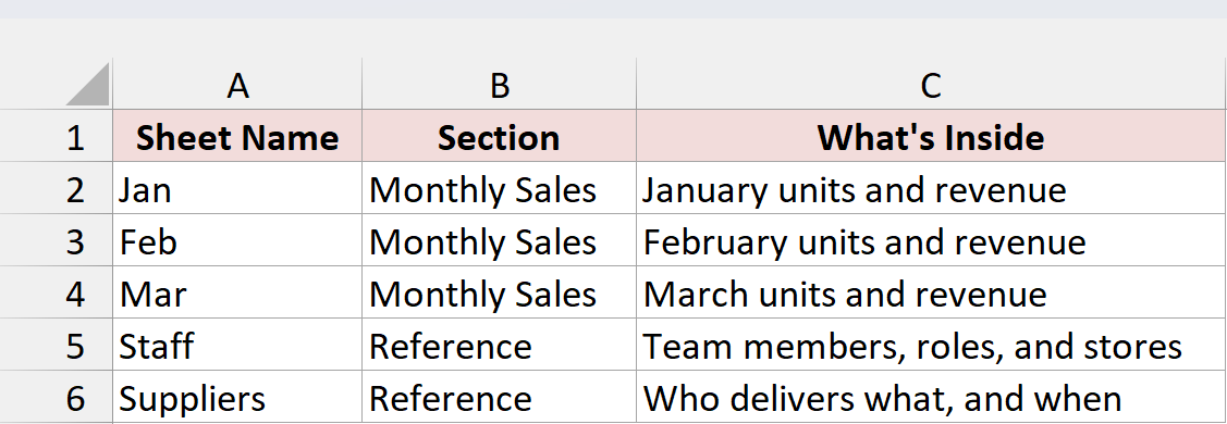
I want each name in column A to open its own sheet when I click it.

Here are the steps to link the sheet names:

1. Select cell A2 (the one that says Jan).

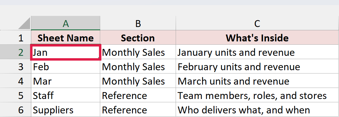
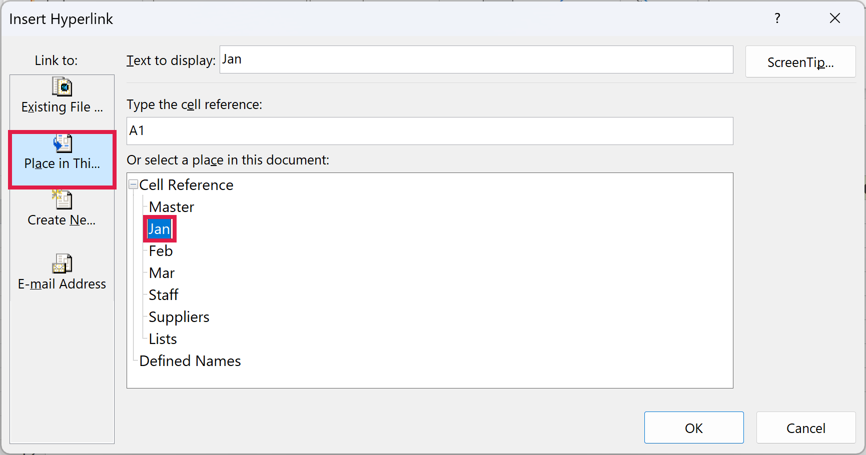
2. Press Ctrl + K (or go to the Insert tab and click Link) to open the Insert Hyperlink dialog box. Click Place in This Document on the left, select Jan under Cell Reference, leave the cell reference as A1, and click OK.

3. Repeat the same steps for A3:A6, picking the matching sheet each time.

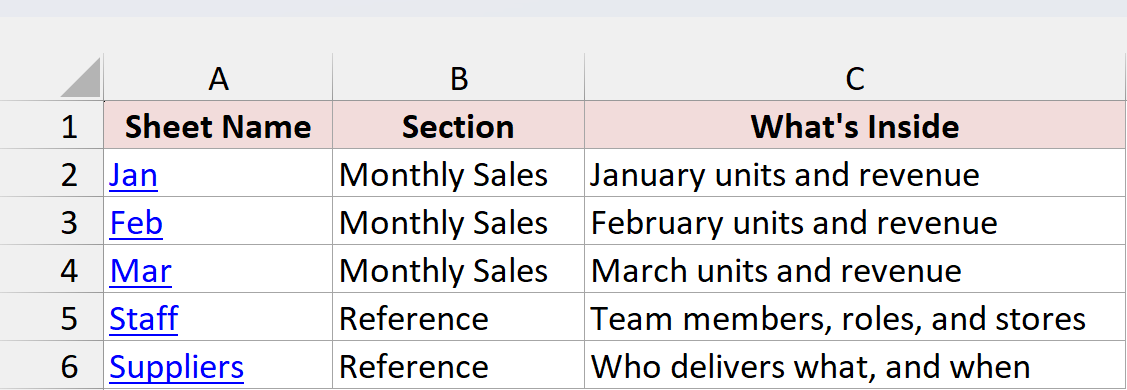
Each sheet name now shows up blue and underlined. Click Staff, and Excel jumps straight to the Staff sheet.

The index gets you to a sheet, but you also need a way back. So I added a Back to Master link to each sheet.

On the Jan sheet, I typed Back to Master in cell E1, pressed Ctrl + K, clicked Place in This Document, and picked Master. Then I did the same on the other sheets.

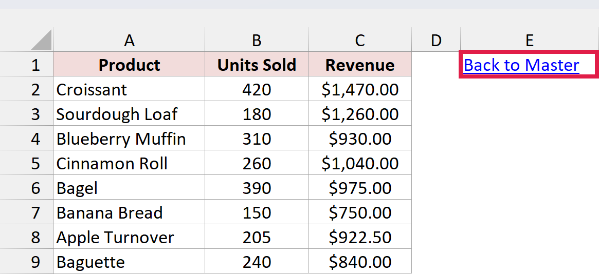
Now you can bounce between the master sheet and any tab without scrolling through the tab strip. Once you’re used to the Ctrl + K shortcut, each link takes a few seconds.

Note: Links made this way remember the sheet name you picked. If you rename a sheet later, its link stops working, and you need to edit the link (right-click it and choose Edit Hyperlink) to point at the new name.

Method #2: Using the HYPERLINK Function

If you’d rather not set up each link by hand, a formula can build them for you. The HYPERLINK function creates a clickable link from whatever sheet name is typed in the cell next to it.

Below I have the same Master sheet, with the sheet names in A2:A6.

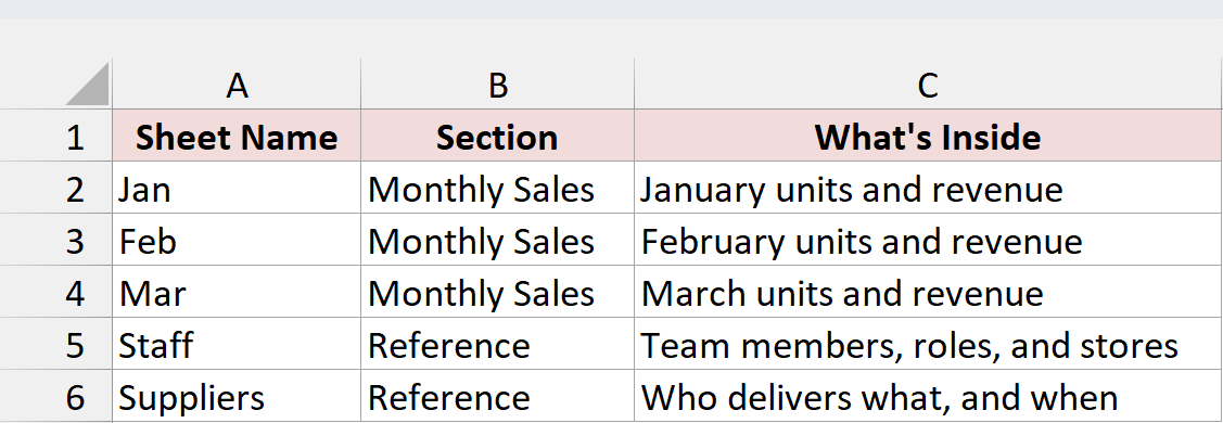
I want a Link column in D that takes me to each sheet. I typed Link in D1.

Here is the formula I entered in D2:

=HYPERLINK("#'"&A2&"'!A1",A2)

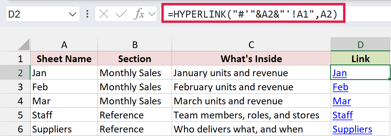
I then copied it down to D6. HYPERLINK doesn’t spill properly here: if you give it A2:A6 in one go, every result shows Jan. So enter it in D2 and copy it down instead.

How does this formula work?

The first argument builds the link location. For row 2, "#'"&A2&"'!A1" becomes #'Jan'!A1.

The # tells Excel the destination is inside this workbook. The single quotes around the sheet name keep the link working if a name has spaces in it, like Q1 Sales. And !A1 is the cell the link lands on.

The second argument, A2, is the text you see in the cell. So D2 shows Jan and takes you to cell A1 of the Jan sheet.

The nice part is that the link reads the name from column A. If you rename a sheet, just type the new name in column A, and the link follows it.

Method #3: Using Tab Colors

The tab strip can do some organizing on its own. Coloring related tabs the same color is the closest thing Excel has to grouping tabs into folders.

Below is the tab strip of the bakery workbook. Master comes first, then three monthly sales sheets, then two reference sheets, and a Lists sheet at the end.

I want the monthly sheets in one color and the reference sheets in another, all sitting right after Master.

Start by putting the tabs in order. Drag each tab left or right until every group sits together after Master. In my workbook they’re already in the right order.

Here are the steps to color a group of tabs:

1. Click the Jan tab, hold the Ctrl key, and click Feb and Mar. All three tabs now look selected, and Excel adds Group next to the file name in the title bar.

2. Right-click any of the selected tabs, go to Tab Color, and pick a color. I went with Green.

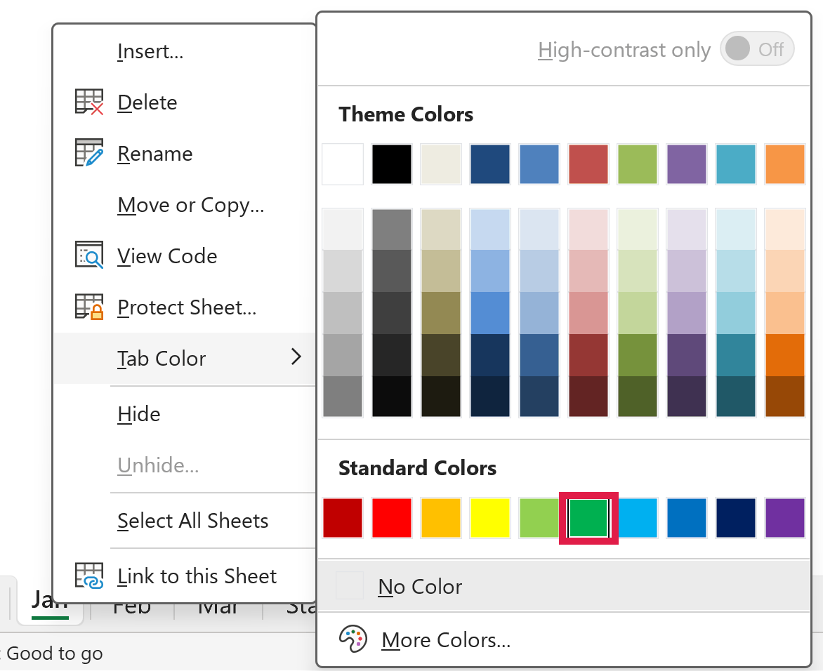
3. Repeat for the other groups. I selected Staff and Suppliers and colored them Blue, then gave Master its own color (Orange) so it stands out.

Now you can tell at a glance which tabs belong together. While a tab is selected, its color only shows as a thin line under the name. Click a different tab to see the full color.

Note: Ctrl-clicking tabs groups them, which means anything you type or delete goes into every grouped sheet at once. Once you’re done coloring, right-click a tab and choose Ungroup Sheets before you edit any cells.

Method #4: Hiding the Helper Sheets

Some tabs exist only to feed other sheets, like a price list or a dropdown list. Nobody needs to open them, so hiding them leaves fewer tabs to scan through.

Below is the bakery workbook’s tab strip. The Lists sheet at the end holds unit prices, and nobody needs to look at it day to day.

I want to hide Lists so the strip only shows Master and the sheets people actually use.

Here are the steps to hide a sheet:

1. Right-click the Lists tab and choose Hide.

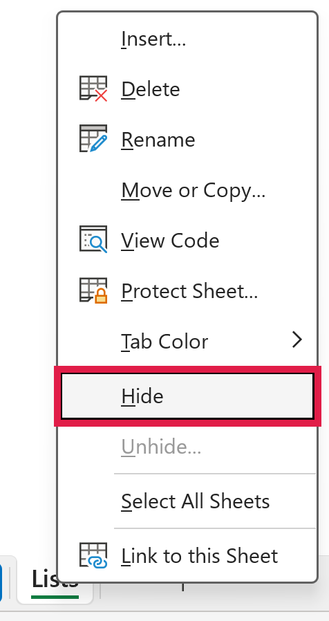
The Lists tab disappears from the strip. Any formulas that use it keep working.

Only hide sheets you never need to click into. A link from your master sheet can’t open a hidden sheet, so clicking it won’t take you there. When you need a hidden sheet again, right-click any tab and choose Unhide to unhide the tab.

Note: A hidden sheet still shows up in the Unhide list. To keep it out of that list too, make it very hidden: press Alt + F11, select the sheet in the Project Explorer, press F4 to open the Properties window, and set Visible to 2 – xlSheetVeryHidden.

Method #5: Using 3D References

Your master sheet can also add up numbers from the sheets under it, so you see the totals without opening every tab.

Below I have the Jan sheet. It lists eight bakery products with their units sold and revenue. Feb and Mar have the exact same layout, with each product in the same row.

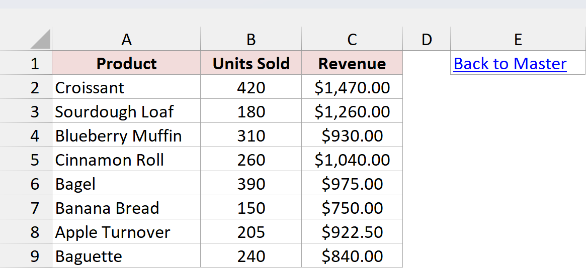
I want the total units sold for each product across all three months on the Master sheet. I typed Product and Q1 Units Sold in F1:G1 and listed the products in F2:F9, in the same order as the month sheets.

Here is the formula I entered in G2:

=SUM(Jan:Mar!B2)

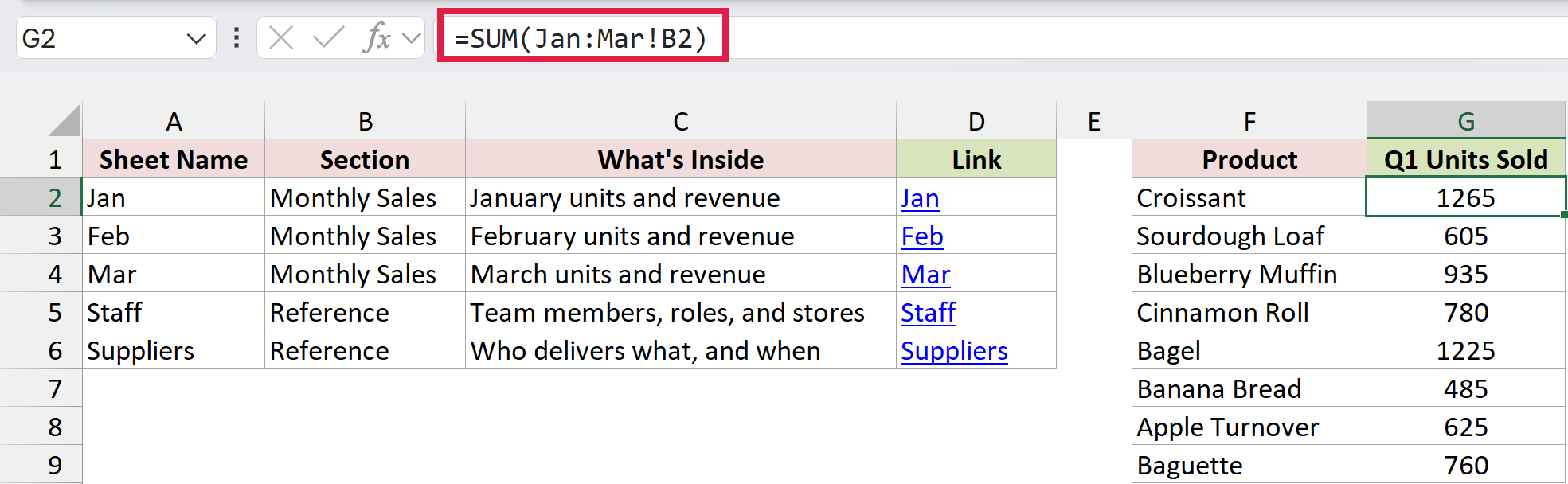
I then copied it down to G9. SUM collapses its range into a single number, so each product needs its own formula.

How does this formula work?

Jan:Mar!B2 is a 3D reference. It means cell B2 on Jan, Mar, and every sheet that sits between them in the tab strip.

So G2 adds up the Croissant units from all three months: 420 + 395 + 450 = 1265. Copy it down, and G3 picks up B3 from each sheet, and so on.

This is where tab order matters. Any sheet you place between Jan and Mar gets included automatically, and any sheet you drag out of that span drops out of the total.

Note: Keep Master outside the Jan-to-Mar span, or it ends up adding its own numbers. Also, 3D references work with SUM, AVERAGE, COUNT, MAX, and MIN, but not with SUMIF, which needs a different approach to use SUMIF across multiple sheets.

Method #6: Using a VBA Macro

If you add or rename tabs every week, keeping the index up to date by hand gets old. A short macro can list every sheet name on the master sheet and link each one, every time you run it.

Below is the bakery workbook’s tab strip. It has Master plus six other sheets, including Lists.

I want column A of the Master sheet to show every visible sheet as a clickable link, in tab order.

Here is the VBA code:

Sub RefreshSheetIndex()
    Dim idx As Worksheet
    Dim sh As Worksheet
    Dim r As Long

    Set idx = ThisWorkbook.Worksheets("Master")

    'Clear the old list in column A (this removes the old links too)
    idx.Range("A2:A" & idx.Rows.Count).ClearContents

    r = 2
    For Each sh In ThisWorkbook.Worksheets
        'Skip the master sheet itself and any hidden sheets
        If sh.Name <> idx.Name And sh.Visible = xlSheetVisible Then
            idx.Cells(r, "A").Value = sh.Name
            idx.Hyperlinks.Add Anchor:=idx.Cells(r, "A"), Address:="", _
                SubAddress:="'" & Replace(sh.Name, "'", "''") & "'!A1"
            r = r + 1
        End If
    Next sh
End Sub

Sub RefreshSheetIndex()
    Dim idx As Worksheet
    Dim sh As Worksheet
    Dim r As Long

    Set idx = ThisWorkbook.Worksheets("Master")

    'Clear the old list in column A (this removes the old links too)
    idx.Range("A2:A" & idx.Rows.Count).ClearContents

    r = 2
    For Each sh In ThisWorkbook.Worksheets
        'Skip the master sheet itself and any hidden sheets
        If sh.Name <> idx.Name And sh.Visible = xlSheetVisible Then
            idx.Cells(r, "A").Value = sh.Name
            idx.Hyperlinks.Add Anchor:=idx.Cells(r, "A"), Address:="", _
                SubAddress:="'" & Replace(sh.Name, "'", "''") & "'!A1"
            r = r + 1
        End If
    Next sh
End Sub

Here are the steps to use this macro:

1. Open the example file and click Enable Editing if Excel shows a Protected View bar.
2. Go to File > Save As and save a copy as an Excel Macro-Enabled Workbook (.xlsm). A regular .xlsx file can’t keep macros.
3. Press Alt + F11 to open the VB Editor, then click Insert > Module.
4. Paste the code above into the new module.

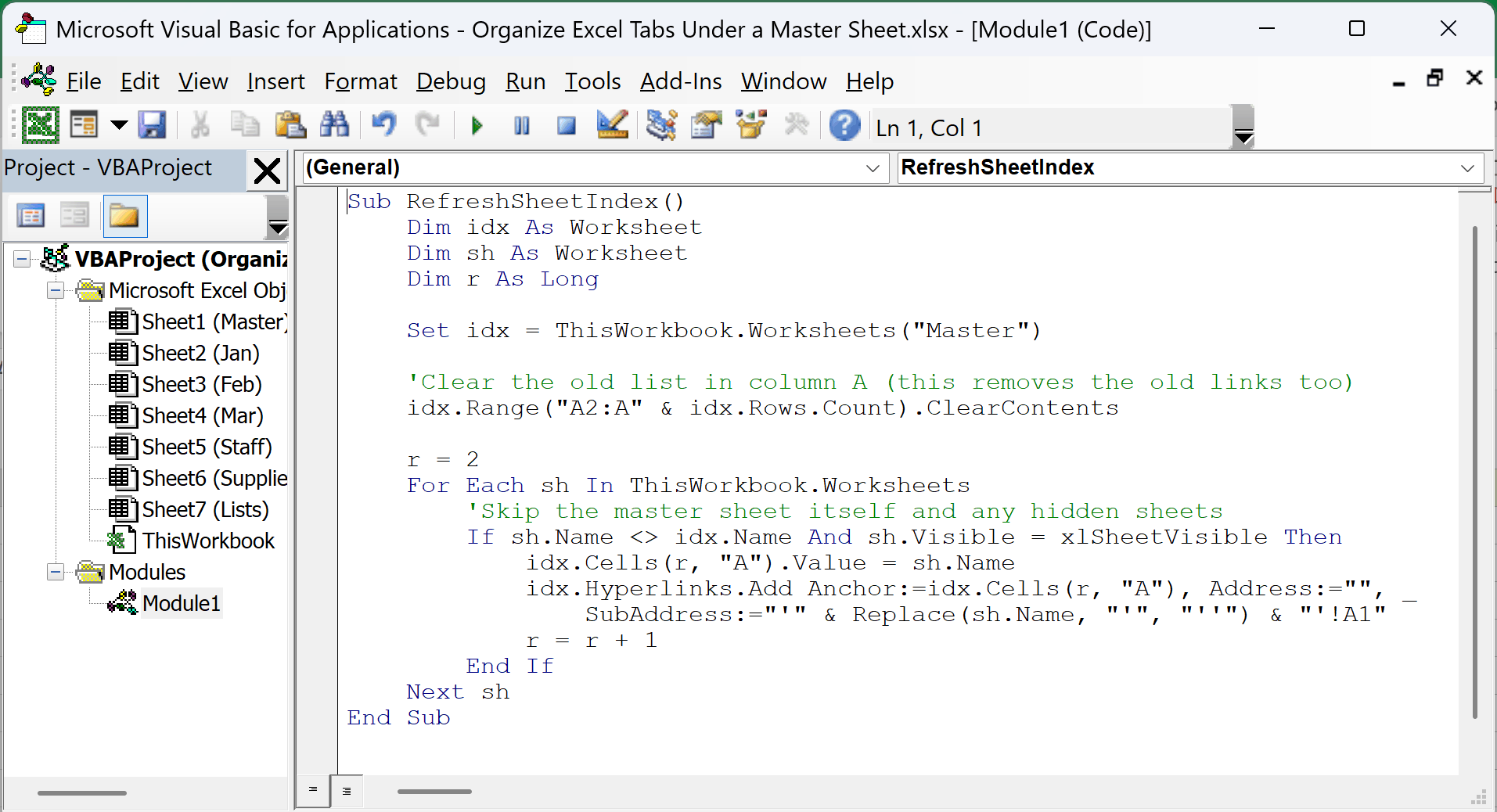
5. Go back to Excel, press Alt + F8, select RefreshSheetIndex, and click Run.

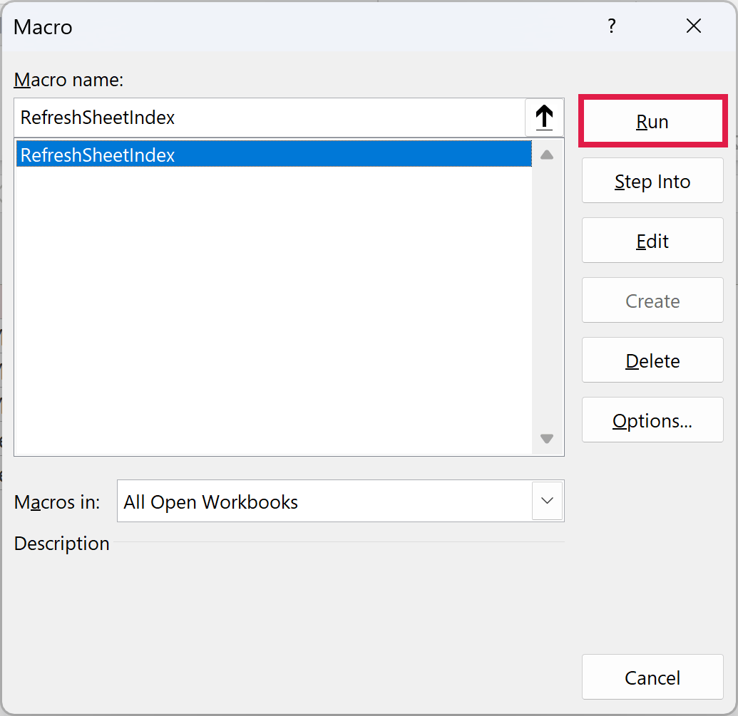
The macro clears column A of Master from row 2 down, then goes through the sheets from left to right. For every visible sheet except Master, it writes the sheet name and turns it into a link to cell A1 of that sheet.

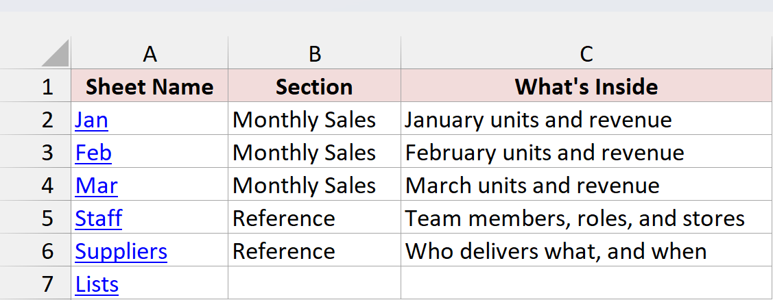
In the example file, the first five names are already there, so the change you’ll see is Lists showing up in A7. Add a new sheet and run the macro again, and its name appears in the list in the same spot as its tab.

Hidden sheets are skipped on purpose, since a link to a hidden sheet wouldn’t go anywhere. The Replace part doubles any apostrophe in a sheet name (like Owner’s Notes), which Excel needs for the link to work.

Note: The macro only rewrites column A. Anything you’ve typed in the columns next to it stays put, so if a new sheet lands in the middle of the list, those descriptions end up on the wrong rows. Use it on a master sheet that only holds the list, or check those columns after each run.

Additional Notes About Organizing Excel Tabs

• Excel has no folders for tabs, so every method here is a workaround. A master sheet with links, plus colored and ordered tabs, is as close as you’ll get without an add-in.
• Right-clicking the tab scroll arrows gives you a quick list. The small arrows at the bottom left of the window open an Activate dialog listing every visible sheet, which is a handy way to switch between tabs in a crowded workbook.
• In Microsoft 365, go to View > Navigation to open a side panel that lists every sheet in the workbook.
• Renaming a sheet affects each method differently. Insert Link links break, HYPERLINK links follow whatever is typed in column A, and 3D references update on their own.

Frequently Asked Questions

Here are a few questions people often ask about organizing tabs in Excel.

Can you put tabs inside another tab in Excel?

No. Excel doesn’t support nested or collapsible tabs. Every worksheet sits on the same level. A master sheet with links to the other tabs is the usual workaround.

Does grouping sheets put them under one tab?

No. When you group worksheets by Ctrl-clicking their tabs, Excel only selects them together so one edit lands on all of them. The group ends as soon as you ungroup or click another tab.

Why does a link on my master sheet stop working?

Usually the sheet it points to was renamed, deleted, or hidden. Links made with Insert Link keep the old sheet name, so edit the link or recreate it.

Do these links work on a Mac or in Excel for the web?

On a Mac, use Cmd + K or Insert > Link. In Excel for the web, Microsoft says HYPERLINK only works with web addresses, and macros don’t run there. If people open the file in a browser, test your links there first.

Conclusion

Excel won’t nest tabs for you, so a master sheet is the next best thing.

In this article, I showed you how to build a clickable index with Insert Link or the HYPERLINK function, color and hide tabs, pull totals together with 3D references, and rebuild the index with a macro.

For most workbooks, I’d start with Insert Link plus a Back to Master link on every sheet.

I hope you found this article helpful.

Other Excel articles you may also like:

• How to Link Cells in Excel (Same Worksheet, Between Worksheets/Workbooks)
• How to Reference Another Sheet Dynamically in Excel