A border makes a chart in Excel stand out and attract the readers’ attention. If you have multiple charts on the same sheet, adding a border also makes them look neat.
In this tutorial, you will learn how to apply an outline border to a chart in Excel.
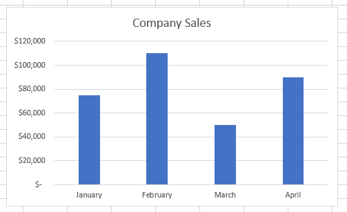
We will use the following chart in our illustration:
Method #1: Add Border to a Chart by Applying a Predefined Quick Style
You can apply a predefined Quick Style border to a chart in Excel.
We use the steps below:
- Click just below the top boundary of the chart to select the Chart Area of the graph.

When the chart is selected, the contextual Format tab on the Ribbon is activated.

- Open the Quick Styles gallery in the Shape Styles group. Hover the mouse pointer over each of the colored outlines to see a live preview in the chart. Select the colored outline that you prefer. In our example, we have chosen the Black outline.

The outline border that you choose is applied to the chart:

Note: The Chart Design and Format contextual tabs appear only when you select a chart. Also, it would only appear when you select one chart. If you select multiple charts at once and try to add borders to all the charts, you won’t be able to do that
Also read: How to Overlay Graphs in Excel
Method #2: Add Border to a Chart Using the Shape Outline Options
We can use the Shape Outline options to apply a border to an Excel chart.
We use the following steps:
- Click just below the top boundary of the chart to select the Chart Area of the graph.

When the chart is selected, the contextual Format tab on the Ribbon is activated.

- Click the Format tab, and in the Shape Styles group, click on the Shape Outline option.

- Hover the mouse pointer over the Weight option and choose a line thickness for the border from the flyout menu.

The outline border is applied to the chart:

Customizing the Chart Outline
If you want more customization of the chart outline, click the More Lines option to open the Format Chart Area pane.
The pane has more options that you can use to customize the line for example adding transparency.
Note: Once you click an option it is applied and the Shape Outline drop-down list is closed. You need to click the Shape Outline button again to reopen the options list if you want to apply more options.
- Click the Shape Outline button to reopen the drop-down list.
- Hover the mouse over the Dashes line styles options on the flyout menu. The options include dashed and dotted styles You will see a live preview in the chart. Choose a line style that appeals to you most.

The line style is applied:

Click More Lines to see advanced options for the line style.
- Click the Shape Outline button and hover the mouse pointer over the Theme Colors buttons or Standard Colors buttons. You get a live preview in the chart. Choose the color you prefer to change the color of the border from Excel’s default gray.

If you do not see the color you want, click More Outline Colors.
The color you choose is applied:

Note: Sometimes you may collaborate with team members in creating a chart. You can apply a Sketched border style to your chart to mark a “draft” or “work in progress” chart. The Sketched border can be converted to straight lines once final changes have been made to the chart
Proceed to the next step if you want to apply a Sketched border to your chart.
- Hover the mouse pointer over the Sketched line style options on the flyout menu. The styles include Curved, Freehand, and Scribble. You will see a live preview in the chart. Choose a line style that appeals to you most.

Click More Lines to see and apply advanced options for the line style.
The outline border is applied:

When the final changes have been made to the graph and approved, you can convert the Sketched border to a straight lines border.
Choose None on the Sketched option flyout menu to convert the sketched border to straight lines.

Also read: How to Resize Charts in Excel
Method #3: Add Border to Charts Using the Format Task Pane
If you want the most control in applying an outline border to a chart, use the options in the Format Task Pane. The Format Task Pane has a wider range of controls to apply and format a chart’s outline border.
The Format Task pane does not obscure your worksheet and remains open until you close the window.
We use the steps below:
- Access the Format Task Pane.
You can access the Format Task Pane in four ways. You can access it by clicking the Format Shape dialog box launcher in the bottom-right corner of the Shape Styles group:

Or
You can also access it by right-clicking the Chart Area and choosing Format Chart Area on the shortcut menu.

Or
Double-click the Chart Area.
Or
Select the Chart Area and press Ctrl +1.
The Format Task Pane is displayed on the right of the Excel window with the options tailored for the Chart Area:

- Click the arrow next to the Border option to open its settings.

- Select the Solid line option and customize it by adjusting its color, transparency, width, and so on.

The outline border is applied to the chart:

Also read: How to Add Axis Titles in Excel?
Method #4: Add Border to Charts Using VBA Macro
Some organizations may specify requirements for the outline borders for charts.
For example, they may want them to have the company colors and be of a certain weight.
You can capture those requirements in a subroutine and assign a keyboard shortcut to the subroutine.
This will save you time and effort in applying outline borders to the organization’s charts.
We use the following steps:
- While in the active worksheet that contains the chart press Alt + F11 to open the Visual Basic Editor.
- Click Insert >> Module to insert a module.

- Copy the following procedure and paste it into the module. Remember to customize it to your requirements.
'Code by Steve from https://spreadsheetplanet.com
Sub ApplyChartOutlineBorder()
    ActiveSheet.ChartObjects("Chart 1").Activate

    With ActiveSheet.Shapes("Chart 1").Line
        .Visible = True
        .Weight = 0.75
        .ForeColor.RGB = RGB(255, 0, 0)
    End With

    ActiveChart.Parent.RoundedCorners = True
End Sub- Save the procedure and save the workbook as a Macro-Enabled Workbook.
- Press Alt + F11 to switch to the active worksheet.
- Press Alt + F8 to open the Macro dialog box.

- Select the applyChartOutlineBorder macro in the Macro name box and click the Options button.
- In the Macro Options dialog box that pops up, create a shortcut key by adding a symbol, number, or letter in the box next to Ctrl.

Note: Be careful that you do not override existing Excel shortcut keys, such as Ctrl + B for bolding. You can prevent this by adding Shift to the shortcut key. In our example, we use Ctrl + Shift + B.

- Click OK to close the Macro Options dialog box.
- Close the Macro dialog box by clicking the close button in the top right corner of the dialog box.
- Press Ctrl + Shift + B to apply the outline border to the chart.

Note: You can use this keyboard shortcut to apply an outline border to charts in other worksheets in the workbook.
The above procedure applies an outline border to one chart at a time. If you have many charts in the workbook, you can use the following procedure that loops through and applies an outline border to the Chart Area of all the charts in the workbook.
'Code by Steve from https://spreadsheetplanet.com
Sub applyOutlineBorderAllCharts()

Dim crtSheet As Worksheet
Dim sht As Worksheet
Dim crt As ChartObject

Application.ScreenUpdating = False
Application.EnableEvents = False

Set crtSheet = ActiveSheet

For Each sht In ActiveWorkbook.Worksheets
  For Each crt In sht.ChartObjects
    crt.Activate
    With ActiveSheet.Shapes(ActiveChart.Parent.Name).Line
        .Visible = msoTrue
        .Weight = 0.75
        .ForeColor.RGB = RGB(255, 0, 0)
    End With
    ActiveChart.Parent.RoundedCorners = True
  Next crt
Next sht

crtSheet.Activate

Application.ScreenUpdating = True
Application.EnableEvents = True

End SubIn this tutorial, we demonstrated four methods that can be used to apply an outline border to a chart in Excel. You can use the method that appeals to you most.
Other Excel articles you may also find useful:
- How to Add Cell Borders in Excel
- Save Excel Chart as Image (High Resolution)
- How to Add a Trendline in Excel Charts?
- How to Add Gridlines in a Chart in Excel?
- How to Remove Gridlines in Excel
- How to Remove Dotted Lines in Excel
- Apply Border to Cells in Excel (Shortcut)
- How to Remove Borders in Excel?
- How to Add Secondary Axis in Excel Charts?