
You have a column of messy bank transaction descriptions in Excel and want categories like Dining or Fuel beside them without tagging each row by hand.
You can categorize text based on keywords by matching words inside each description, but overlapping keywords need an order so the right category wins.
I’ll show you XLOOKUP, IFS, INDEX and MATCH, a TEXTJOIN formula for multiple categories, and Power Query for data you refresh.
Method #1: Using XLOOKUP and SEARCH
I’d start with XLOOKUP. You can keep the keywords in a separate table and return the category for the first match.
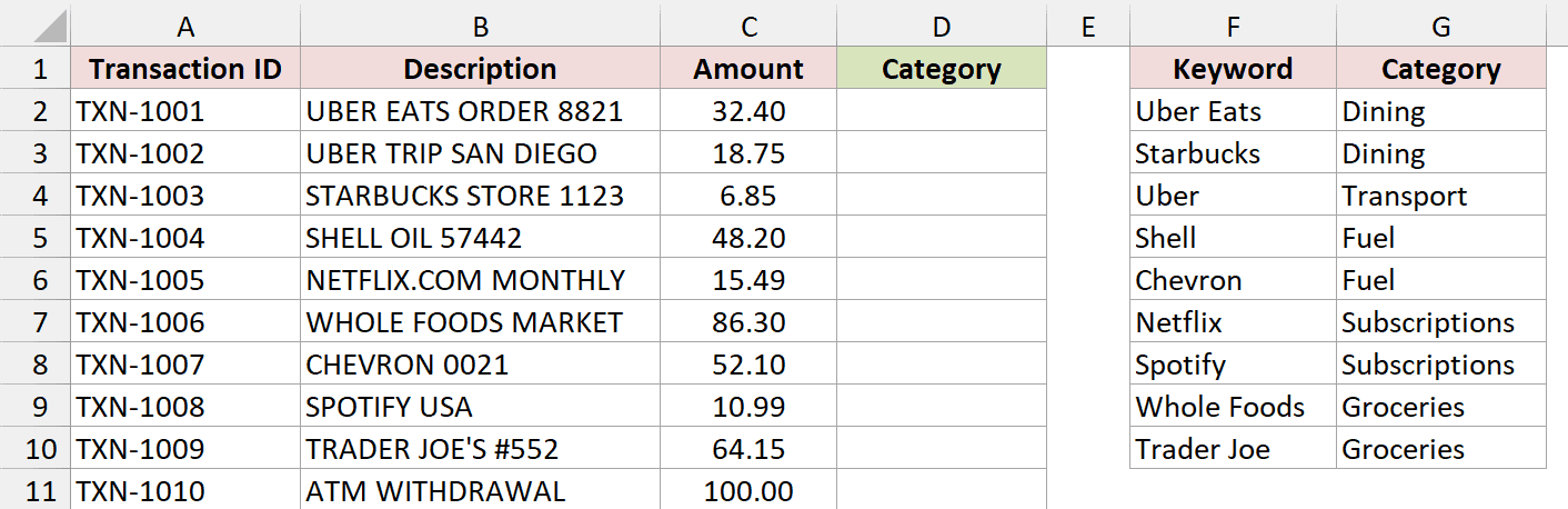
Below I have a dataset of bank transactions on the XLOOKUP sheet, with Transaction ID, Description, and Amount in columns A, B, and C.
The keyword table is in F1:G10.
You want a category in column D for each description in B2:B11, using the keywords in F2:F10 and categories in G2:G10.
Enter this formula in D2, then copy it down to D11:
=XLOOKUP(TRUE,ISNUMBER(SEARCH($F$2:$F$10,B2)),$G$2:$G$10,"Other")
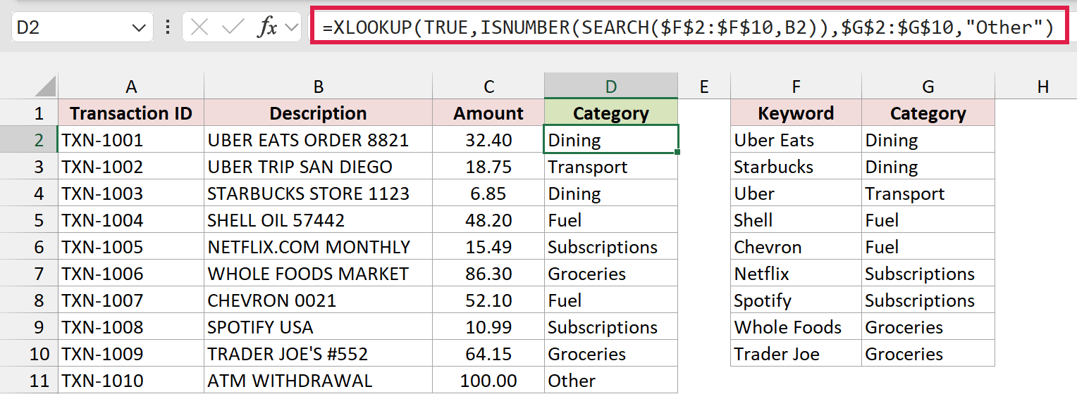
TXN-1001 returns Dining, TXN-1002 returns Transport, and TXN-1010 returns Other because its description doesn’t contain a listed keyword.
The formula checks one description against the whole keyword list.
Giving it B2:B11 instead of B2 won’t make it spill, so you copy it down for each row.
How does this formula work?
In D2, you’re checking “UBER EATS ORDER 8821” against the 9 keywords in the table.
SEARCH($F$2:$F$10,B2) uses SEARCH to look for each keyword inside B2. It returns 9 results, one for each keyword.
A match returns its starting position. Both “Uber Eats” and “Uber” return 1. Keywords that aren’t found return a #VALUE! error.
ISNUMBER turns those results into TRUE or FALSE. The first and third entries in the keyword list return TRUE. The others return FALSE.
XLOOKUP finds the first TRUE and returns the category at that position in G2:G10. The first match is “Uber Eats”, so D2 returns Dining.
The fourth argument, “Other”, handles descriptions with no match. That’s why TXN-1010, “ATM WITHDRAWAL”, returns Other.
Keyword order matters. “UBER EATS ORDER 8821” contains both “Uber Eats” and “Uber”, but “Uber Eats” sits above “Uber”, so Dining wins over Transport.
Put specific keywords above general ones. SEARCH also ignores case, so “Uber” matches “UBER”.
You need Microsoft 365, Excel 2021, or later for XLOOKUP. Older versions show a #NAME? error. Use Method #3 instead.
Method #2: Using the IFS Function
For a short, fixed list, you can put the keywords directly inside the formula. The IFS function checks the conditions in order.
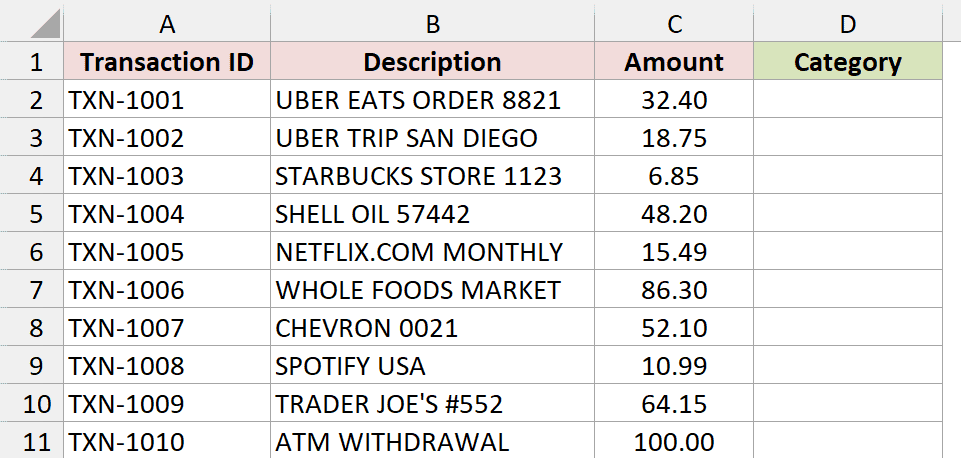
Below I have a dataset of bank transactions on the IFS sheet, with transaction IDs, descriptions, and amounts in columns A:C.
You want to categorize B2:B11 in column D.
This sheet has no separate keyword table. You’ll enter each keyword and its category in the formula below.
Enter this formula in D2, then copy it down to D11:
=IFS(OR(ISNUMBER(SEARCH({"Uber Eats","Starbucks"},B2))),"Dining",ISNUMBER(SEARCH("Uber",B2)),"Transport",OR(ISNUMBER(SEARCH({"Shell","Chevron"},B2))),"Fuel",OR(ISNUMBER(SEARCH({"Netflix","Spotify"},B2))),"Subscriptions",OR(ISNUMBER(SEARCH({"Whole Foods","Trader Joe"},B2))),"Groceries",TRUE,"Other")
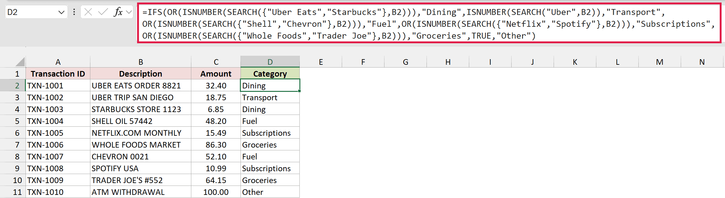
You get the same categories as Method #1, including Dining for TXN-1001 and Other for TXN-1010.
How does this formula work?
IFS checks each condition in order and returns the value paired with the first condition that is TRUE.
The first condition checks for “Uber Eats” or “Starbucks”. SEARCH looks for both keywords inside B2, and ISNUMBER marks each match as TRUE.
OR returns TRUE if either keyword matches, so IFS returns Dining. The curly braces group multiple keywords into one test.
The “Uber” condition checks only one keyword, so it doesn’t need OR. A match returns Transport.
The Dining test comes first, so “Uber Eats” gets Dining before the more general “Uber” test can return Transport.
The remaining OR tests return Fuel for “Shell” or “Chevron”, Subscriptions for “Netflix” or “Spotify”, and Groceries for “Whole Foods” or “Trader Joe”.
The last pair, TRUE,"Other", catches anything the earlier tests missed. Without a keyword match, you get Other.
Adding a keyword means editing the formula, and it gets long quickly. With more than a handful of categories, I’d use Method #1.
IFS needs Excel 2019, Excel 2021 or later, or Microsoft 365.
Method #3: Using INDEX and MATCH (Older Excel Versions)
If your Excel version doesn’t have XLOOKUP, you can use INDEX and MATCH with the same keyword table. The first matching keyword still wins.
Below I have another dataset of bank transactions on the INDEX MATCH sheet, with transaction IDs, descriptions, and amounts in columns A:C.
The keyword table is in F1:G10.
You want a category in D2:D11 for each description in B2:B11, using the keywords in F2:F10 and categories in G2:G10.
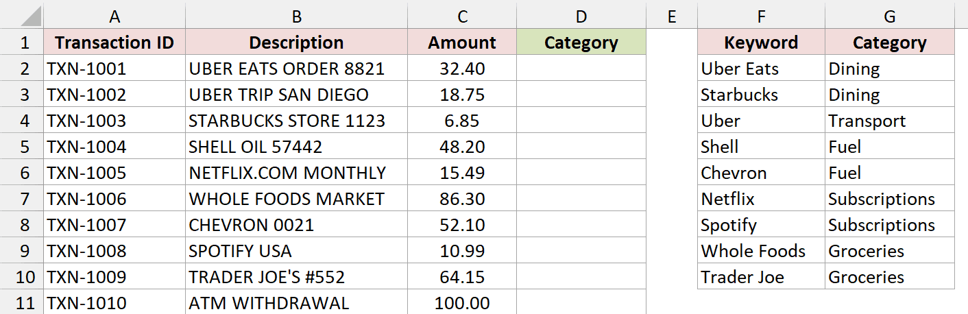
Note: In Excel 2019 and earlier, confirm this array formula with Ctrl + Shift + Enter instead of Enter. Excel adds curly braces around it. In Microsoft 365, Enter is enough.
Enter this formula in D2 using the key combination for your version, then copy it down to D11:
=IFERROR(INDEX($G$2:$G$10,MATCH(TRUE,ISNUMBER(SEARCH($F$2:$F$10,B2)),0)),"Other")
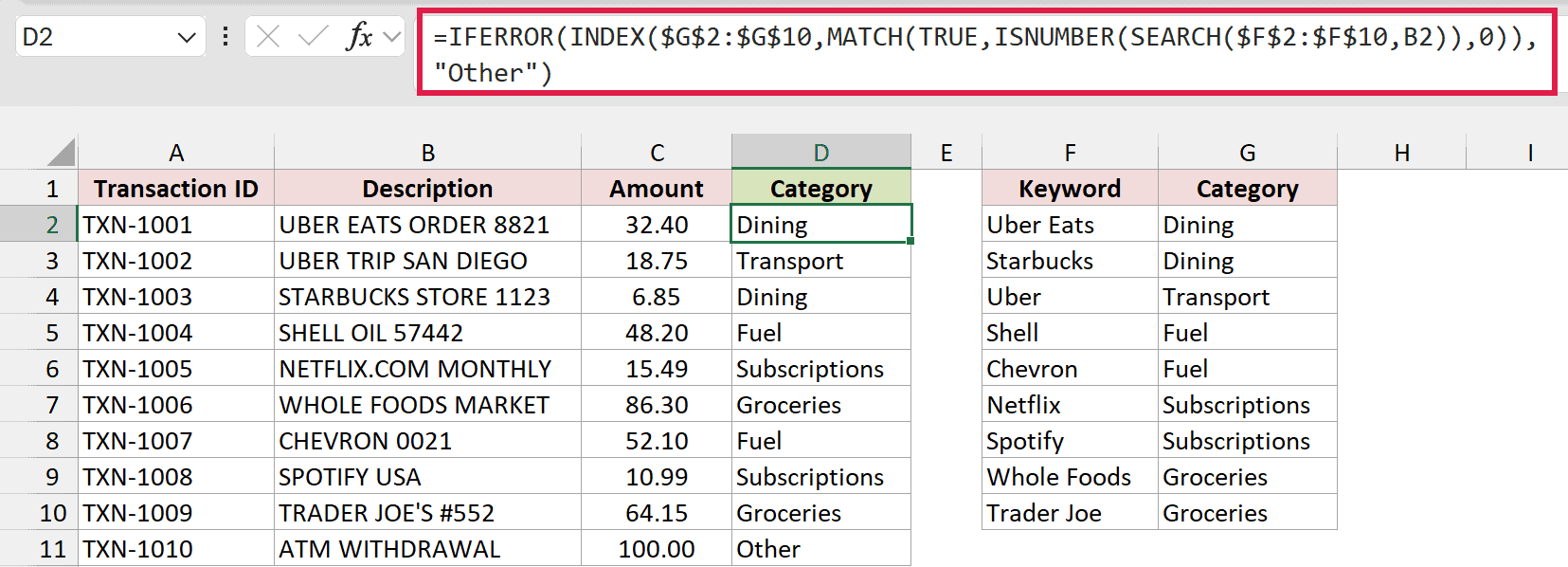
You get the same results as Method #1. TXN-1001 returns Dining, while TXN-1010 returns Other.
How does this formula work?
ISNUMBER(SEARCH($F$2:$F$10,B2)) builds the same TRUE/FALSE list as Method #1, marking the keywords found in the description.
MATCH(TRUE,...,0) returns the position of the first TRUE. For B2, “UBER EATS ORDER 8821”, that position is 1.
INDEX returns the category at that position in G2:G10, so D2 gets Dining.
When no keyword matches, MATCH returns #N/A. IFERROR replaces that error with “Other”, as you see for “ATM WITHDRAWAL”.
Method #4: Using TEXTJOIN and FILTER (Multiple Categories)
Sometimes you need several categories for one cell, such as feedback about a late delivery and a damaged box. Methods #1 to #3 stop at the first match.
This formula returns every matching topic and joins them in one cell.
Below I have a dataset of customer feedback on the Multiple Categories sheet, with Feedback ID in column A and comments in B2:B11.
The keyword table is in E1:F10.
You want the matching topics in column C, using the keywords in E2:E10 and topics in F2:F10.
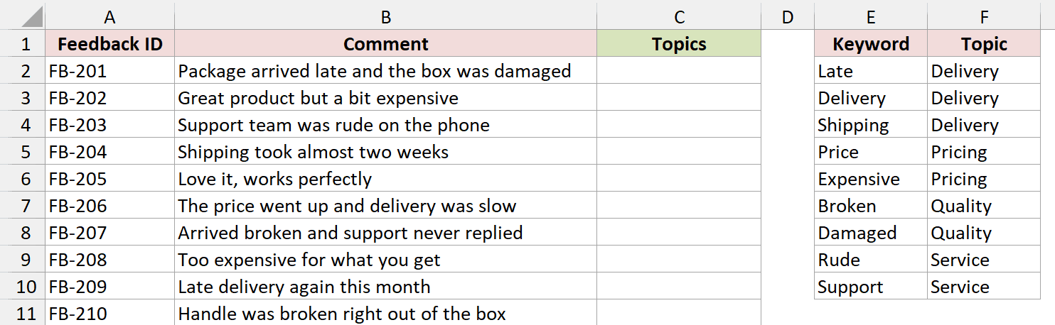
Enter this formula in C2, then copy it down to C11:
=TEXTJOIN(", ",TRUE,UNIQUE(FILTER($F$2:$F$10,ISNUMBER(SEARCH($E$2:$E$10,B2)),"Untagged")))
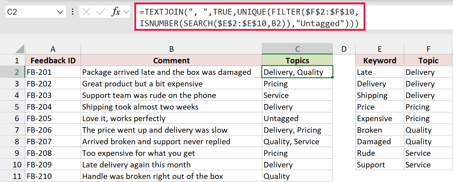
C2 returns “Delivery, Quality” for FB-201, “Package arrived late and the box was damaged”. C6 returns Untagged for FB-205, “Love it, works perfectly”.
The formula works on one comment at a time, so you copy it down for each row.
How does this formula work?
ISNUMBER(SEARCH($E$2:$E$10,B2)) marks which keywords appear in B2. Here, “Late” and “Damaged” match the comment.
FILTER returns the topic in F2:F10 for each TRUE, so it returns Delivery for “Late” and Quality for “Damaged”.
FILTER’s third argument, “Untagged”, handles comments with no matching keywords. That’s the result for FB-205.
UNIQUE removes repeated topics. FB-203, “Support team was rude on the phone”, matches both “Rude” and “Support”, which map to Service, so you get Service once.
TEXTJOIN joins the remaining topics with a comma and a space.
Topics follow the keyword table’s order, rather than their order in the comment. FB-206, “The price went up and delivery was slow”, returns “Delivery, Pricing”.
FILTER and UNIQUE need Microsoft 365, Excel 2021, or later.
Method #5: Using Power Query
For a monthly bank export or other data you re-import often, you can use Power Query to categorize transactions when you refresh the query.
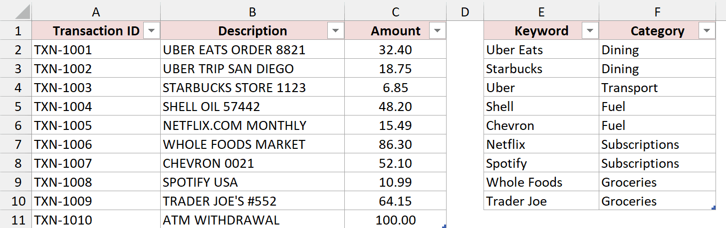
On the Power Query Source sheet, transactions are in A1:C11, and the keyword table is in E1:F10. You want a category beside each description.
Both ranges are already Excel Tables named Transactions and Keywords. Power Query needs Tables. If your data isn’t in one, select it and press Ctrl + T first.
Here are the steps to categorize the transactions with Power Query:
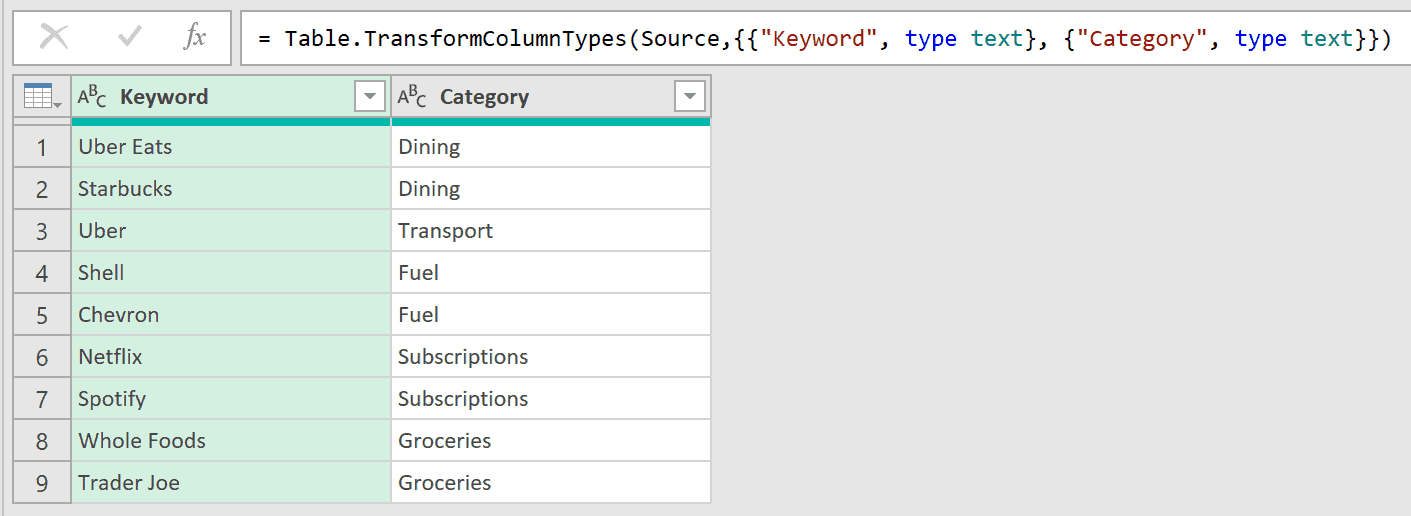
- Select any cell in the Keywords table. On the Data tab, click From Table/Range to open the keyword table in the Power Query Editor.
- On the Home tab, click the Close & Load drop-down, then Close & Load To. In the Import Data dialog, select Only Create Connection and click OK.
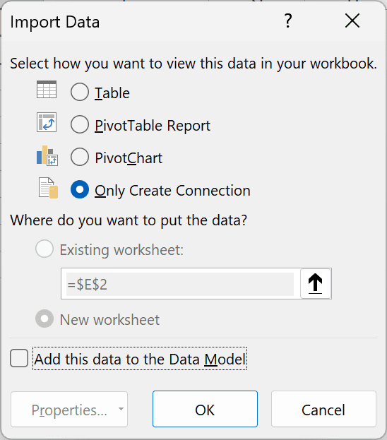
This keeps the keyword list available to Power Query without adding another sheet.
- Select any cell in the Transactions table. On the Data tab, click From Table/Range to open the transactions in the Power Query Editor.
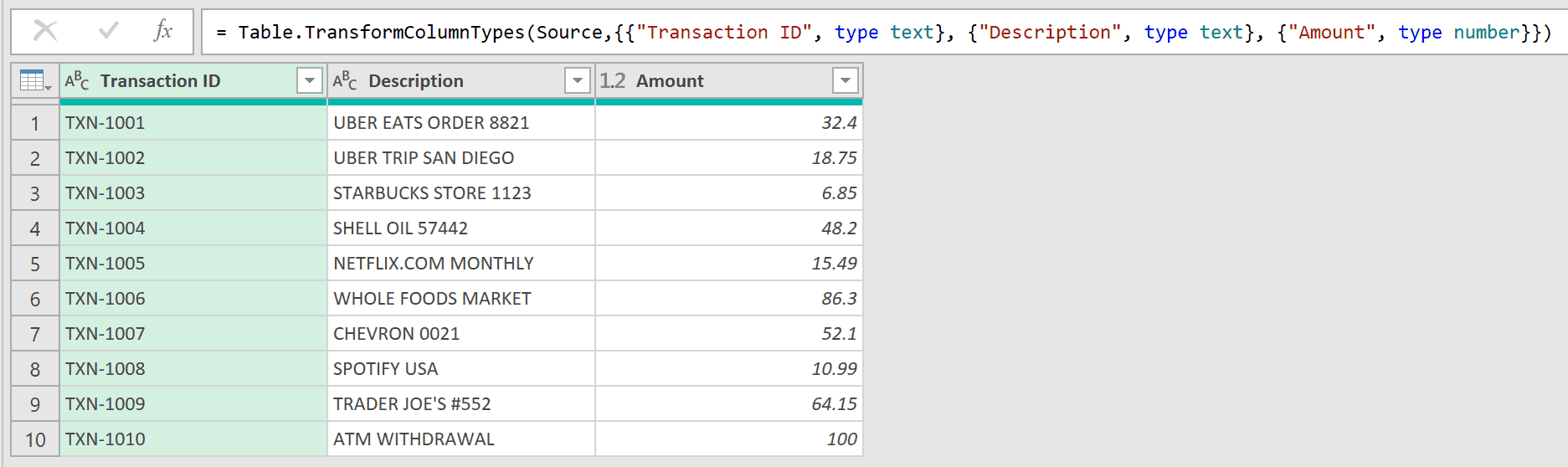
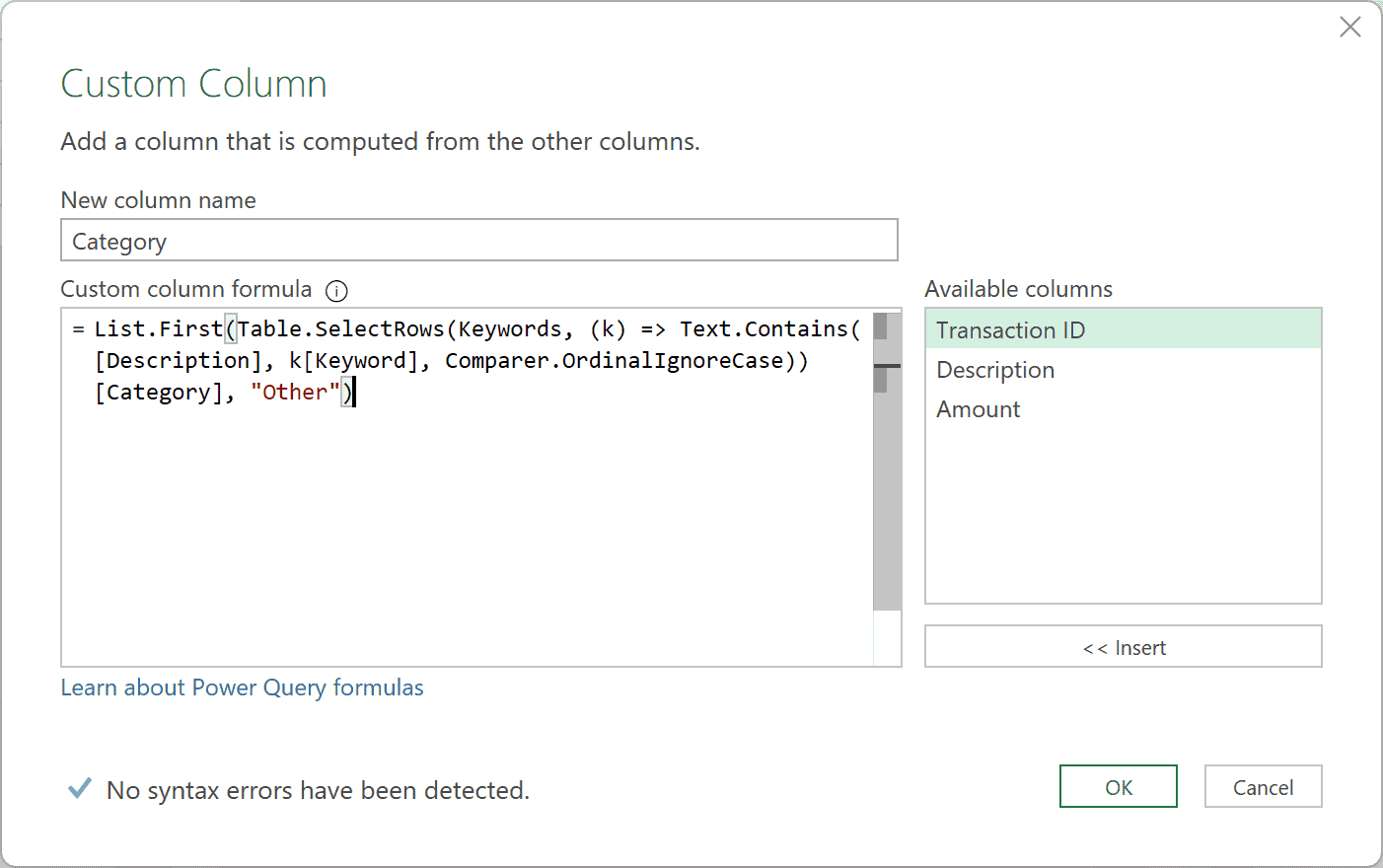
- On the Add Column tab, click Custom Column. Name the new column Category and enter the formula below, then click OK.
List.First(Table.SelectRows(Keywords, (k) => Text.Contains([Description], k[Keyword], Comparer.OrdinalIgnoreCase))[Category], "Other")
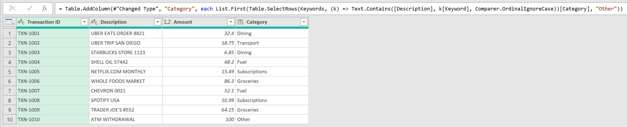
- The Category column now shows the category for each transaction. Check the results: UBER EATS ORDER 8821 returns Dining, and ATM WITHDRAWAL returns Other.
- On the Home tab, click Close & Load to load the categorized transactions into a new table on a new sheet.
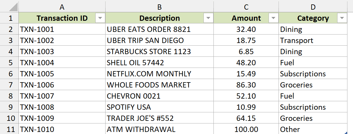
The loaded table has the same categories as Method #1. Your original data stays unchanged.
How does this formula work?
For each transaction, Table.SelectRows keeps only the rows in Keywords whose keyword appears in that transaction’s Description.
Text.Contains checks whether the keyword appears in the description. Comparer.OrdinalIgnoreCase makes it ignore case. Without that argument, Text.Contains is case-sensitive.
[Category] pulls the category column from the matching rows. List.First takes the first category, or “Other” if the list is empty.
As with Method #1, the first match in the keyword table wins. Keep “Uber Eats” above “Uber” so the food order returns Dining.
Refresh is manual. After adding keywords or new transactions, go to Data > Refresh All to update the categorized table.
Additional Notes About Categorizing Text Based on Keywords in Excel
Keep these matching rules in mind when adapting the formulas to your own text:
- SEARCH finds partial matches anywhere in the text. “Shell” also matches “SHELLFISH SHACK”. To check whole words separated by spaces, use
SEARCH(" "&$F$2:$F$10&" "," "&B2&" "). This adds spaces around both the keyword and description, but misses keywords next to punctuation. - SEARCH ignores case. For an exact case match, replace SEARCH with FIND in any of the worksheet formulas.
- The formulas use fixed ranges such as $F$2:$F$10. If you add keywords below row 10, extend the ranges or convert the list to an Excel Table and use references that grow with it.
- SEARCH treats ? and * as wildcards. To find a literal question mark or asterisk, put a tilde (~) before it in the keyword.
Frequently Asked Questions
Here are answers to a few questions you may have when setting up your categories.
How do I leave the cell blank when no keyword matches?
Replace “Other” with "" (two double quotes) in the formula.
Can the keyword table be on a different sheet?
Yes. Point the ranges at that sheet, such as Keywords!$A$2:$A$10 and Keywords!$B$2:$B$10, keeping the dollar signs.
How do I count how many transactions fall in each category?
Use COUNTIF on the result column. For this data, =COUNTIF(D2:D11,"Fuel") returns 2.
Conclusion
I’ve shown you five ways to categorize text based on keywords, and I recommend Method #1 with XLOOKUP as your default.
Use Method #4 when one cell needs several categories. I hope you found this article helpful.
Other Excel articles you may also like:
