
The GAMMA.INV function in Excel returns the value at a chosen cumulative probability in a gamma distribution.
For a task-duration model, that value is the time within which the chosen share of tasks should finish.
GAMMA.DIST works in the opposite direction, turning a value into a probability. GAMMA.INV needs the distribution’s shape and scale before it can calculate a threshold.
In this article, I’ll show you how to set completion thresholds, estimate shape and scale from recorded lead times, and build rainfall ranges.
GAMMA.INV Function Syntax in Excel
GAMMA.INV takes these required arguments:
=GAMMA.INV(probability,alpha,beta)
- probability is the cumulative share at or below the returned value. Use a probability from 0 up to, but excluding, 1.
- alpha is the positive shape parameter, which controls the distribution’s shape.
- beta is the positive scale parameter. It uses the same units as the returned value, such as days or inches.
Beta is a scale, not a rate. The distribution’s mean is its shape multiplied by its scale.
GAMMA.INV is available in Excel 2010 and later.
When to Use GAMMA.INV Function
- Set a completion threshold for tasks modeled with a gamma distribution.
- Calculate rainfall percentiles and compare the median with the mean.
- Estimate distribution parameters from recorded lead times, then calculate a planning threshold.
- Build a central range with a dry-end and wet-end boundary.
- Convert random probabilities into simulated positive durations.
Example 1: Set Task Completion Thresholds
Let’s start with construction tasks whose durations have different shapes and scales.
Below is the dataset with tasks, shape and scale inputs, a confidence-level card, and columns for average days and completion thresholds.
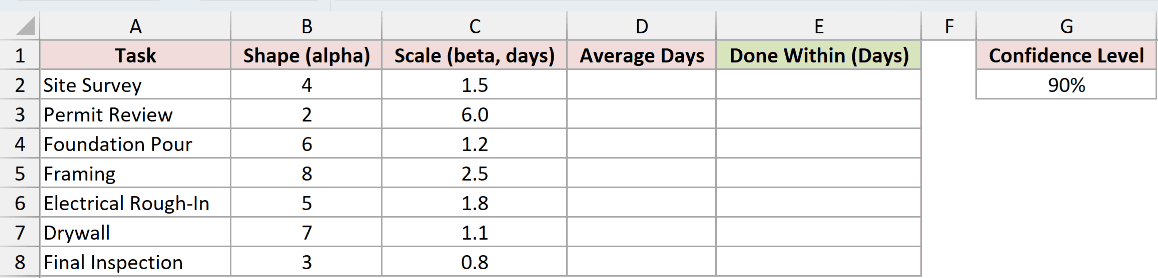
We want the duration within which 90% of each task’s modeled outcomes should finish, alongside its average duration.
First, enter the average-days formula in D2:
=B2:B8*C2:C8
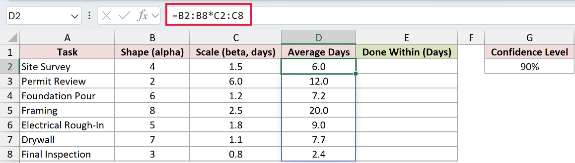
Multiplying each shape by its scale spills the model averages into D2:D8. Permit Review has an average of 12.0 days.
These range formulas spill in Excel 2021, Excel 2024 and Microsoft 365. In Excel 2019 and earlier, use individual row references and fill down.
Now enter the completion-threshold formula in E2:
=GAMMA.INV(G2,B2:B8,C2:C8)
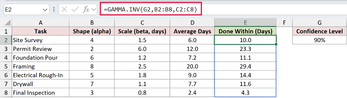
G2 holds the shared probability. Excel pairs each row’s shape and scale, then spills its threshold into E2:E8.
Permit Review returns 23.3 days, compared with its 12.0-day average. The average alone doesn’t describe how long the slower outcomes can take.
Site Survey returns 10.0 days, while Framing returns 29.4 days. Each threshold describes the duration of that individual task.
Pro Tip: The card’s Confidence Level is the modeled share finishing within the threshold. It isn’t a confidence interval for the average duration.
Example 2: Compare Rainfall Percentiles and the Mean
A percentile ladder makes the long upper tail easier to see.
Below is the dataset with cumulative probabilities, a shape-and-scale card, rainfall result cells, a round-trip check column, and a labeled average cell.
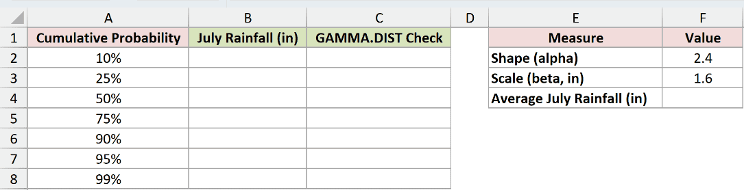
We want July rainfall thresholds at each listed probability, then check those thresholds and compare the median with the mean.
Enter the percentile formula in B2:
=GAMMA.INV(A2:A8,F2,F3)
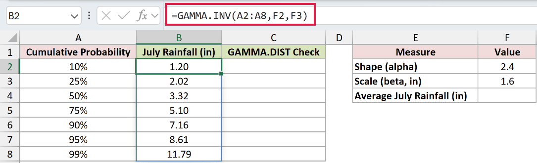
The formula uses the same shape and scale for every probability, spilling rainfall thresholds into B2:B8.
The 50% threshold, or median, is 3.32 inches. The 90% threshold is 7.16 inches, and the 99% threshold reaches 11.79 inches.
To verify the conversion, enter this round-trip check in C2:
=GAMMA.DIST(B2:B8,F2,F3,TRUE)
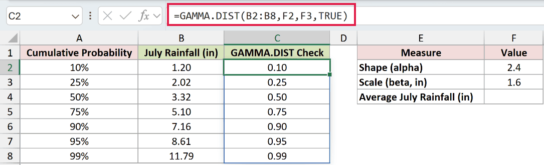
Column C is a round-trip check, not another rainfall answer. GAMMA.DIST converts the calculated thresholds back into cumulative probabilities using the same parameters.
The check beside the median displays 0.50, and the check beside the highest threshold displays 0.99, matching their original probabilities.
Now calculate the model’s mean in F4:
=F2*F3
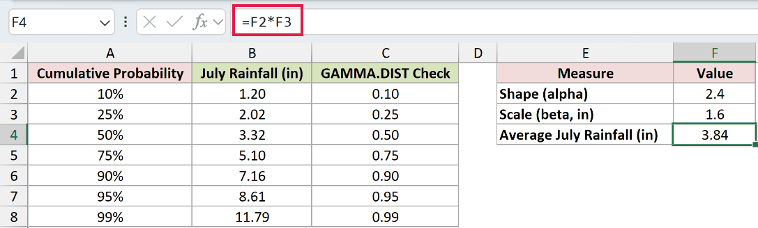
The mean is 3.84 inches, above the 3.32-inch median. The long wet-weather tail pulls the mean upward, so the mean and median aren’t interchangeable.
Example 3: Estimate Shape and Scale From Data
Recorded lead times can supply estimates for the shape and scale.
Below is the dataset with purchase-order IDs and lead times in columns A and B. The card in columns D and E has labels for estimates and the threshold.
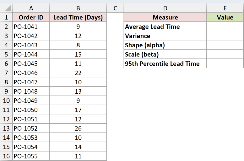
We want to estimate a gamma model from these lead times and calculate its 95th percentile.
Calculate the average in E2:
=AVERAGE(B2:B16)
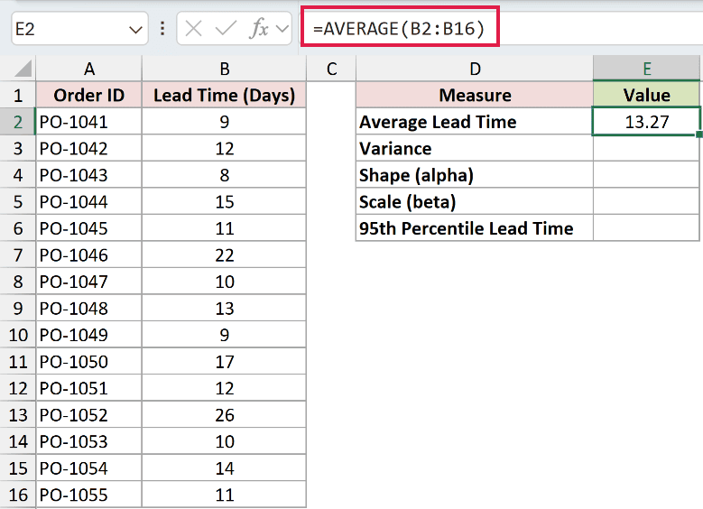
The average lead time displays 13.27 days.
Calculate the sample variance in E3:
=VAR.S(B2:B16)
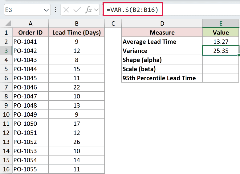
The variance displays 25.35 in squared days. It measures the spread used to estimate the model’s shape and scale.
Estimate the shape in E4:
=E2^2/E3
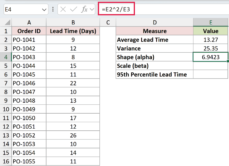
Squaring the mean and dividing by the variance returns a shape of 6.9423.
Estimate the scale in E5:
=E3/E2
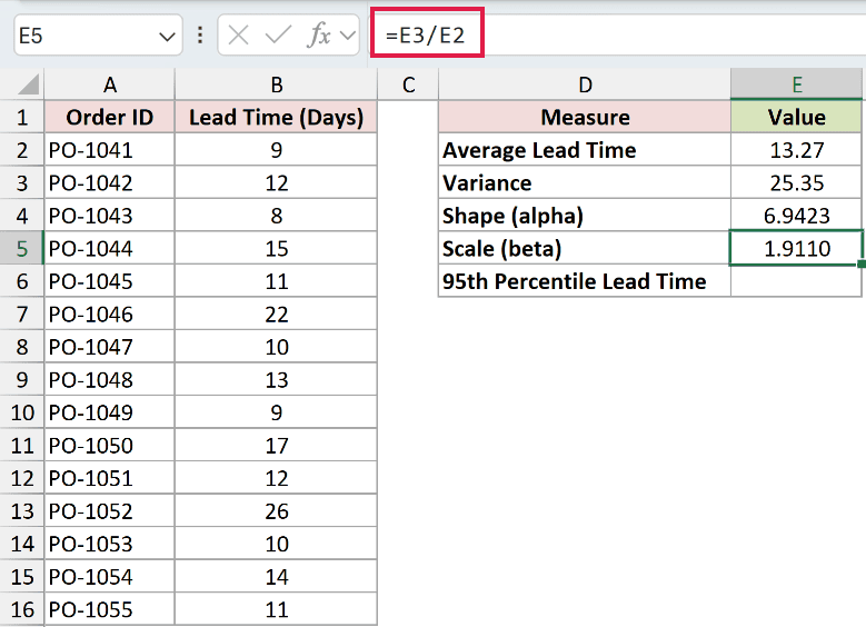
Dividing the variance by the mean returns a scale of 1.9110 days. Together, these estimates match the model’s mean and variance to the sample summaries.
Finally, calculate the threshold in E6:
=GAMMA.INV(0.95,E4,E5)
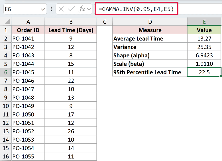
The fitted model’s 95th percentile displays 22.5 days. Under that model, 95% of lead times fall at or below the calculated threshold.
This estimates a percentile from a distribution. PERCENTILE.INC instead calculates a percentile directly from the recorded observations, without fitting a gamma model.
Pro Tip: Reference the calculated cells instead of retyping their displayed, rounded values. Estimating shape and scale doesn’t establish that the gamma distribution fits your data well.
Example 4: Build a Central Rainfall Range
A monthly rainfall range needs both a lower and an upper boundary.
Below is the dataset with monthly shape and scale inputs, a coverage card, and labeled columns for the dry-year low and wet-year high.
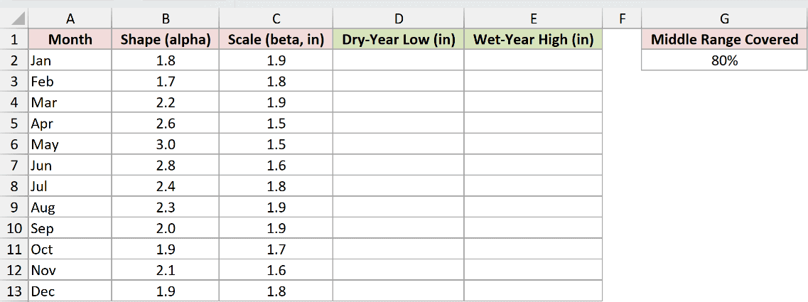
We want a range covering the middle 80% of each month’s modeled rainfall, leaving equal shares outside either end.
Enter the lower-bound formula in D2:
=GAMMA.INV((1-G2)/2,B2:B13,C2:C13)
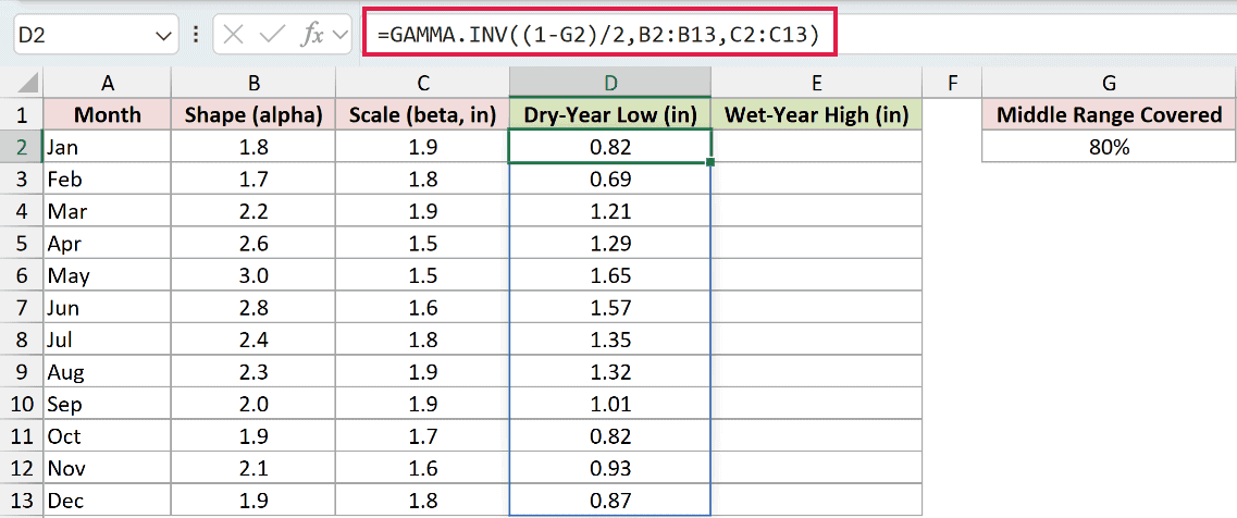
The probability calculation splits the uncovered share equally between the tails. Excel then spills the lower thresholds into D2:D13.
January’s lower boundary displays 0.82 inches, and February’s displays 0.69 inches.
Enter the upper-bound formula in E2:
=GAMMA.INV(1-(1-G2)/2,B2:B13,C2:C13)
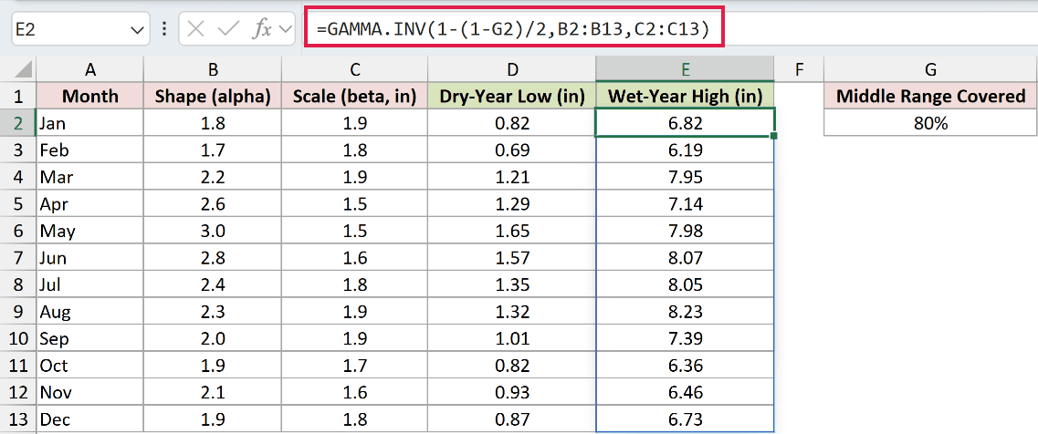
This uses the cumulative probability at the upper edge and spills the upper thresholds into E2:E13.
January’s modeled range is 0.82 to 6.82 inches. February’s is 0.69 to 6.19 inches.
The low end stays positive. A symmetric range from NORM.INV can extend below zero for skewed rainfall data, where negative rainfall wouldn’t make sense.
These are ranges for rainfall outcomes under the supplied models. Each range describes how much rainfall that month could receive.
Example 5: Simulate Positive Task Durations
The same inverse calculation can turn random probabilities into simulated durations.
Below is the dataset with run numbers, fixed random-number inputs, a duration column, and a parameter card with labeled expected-average and simulated-average cells.
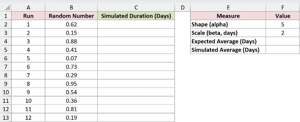
We want to convert each probability into a duration, then compare the simulated average with the model’s expected average.
Enter the simulation formula in C2:
=GAMMA.INV(B2:B13,F2,F3)
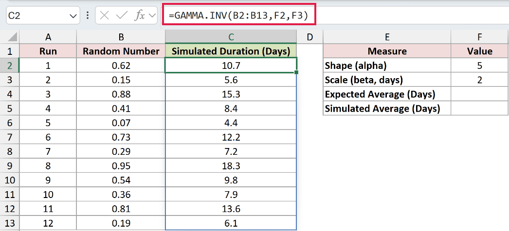
The results spill into C2:C13. Each input selects a position in the gamma distribution, so higher probabilities produce longer durations.
The fixed input 0.62 produces 10.7 days, while 0.95 produces 18.3 days. These inputs are saved values so the example and screenshot stay reproducible.
Calculate the expected average in F4:
=F2*F3
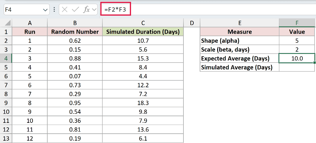
The model’s expected average is 10.0 days.
Calculate the simulated average in F5:
=AVERAGE(C2:C13)
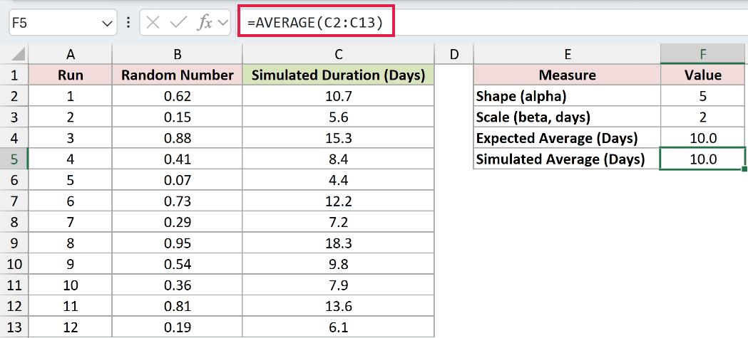
The simulated average also displays 10.0 days. Matching displayed averages doesn’t mean they are exactly equal or that another set of random inputs will match.
For a live simulation, replace the fixed inputs with values generated by RAND or RANDARRAY. In automatic calculation mode, they recalculate on every edit and when you press F9.
GAMMA.INV itself isn’t volatile. The changing random inputs make its simulated durations change.
Tips & Common Mistakes
- If your source supplies an event rate, convert it to its reciprocal before using it as beta. Entering the rate directly changes the model.
- A probability of 0 returns 0. A probability of 1 or above returns
#NUM!; negative probabilities also return#NUM!. - Alpha and beta must both be positive. Check the parameter cells before calculating thresholds.
- Occupied cells in the destination range cause
#SPILL!. An added@can force a range expression to return a single value. - GAMMA.INV turns a cumulative probability into a threshold. GAMMA.DIST turns a threshold into a cumulative probability when its cumulative argument is TRUE.
- A threshold is only useful when the supplied shape and scale describe the process you’re planning for.
Try changing the target probability in the task-duration example while keeping the shape and scale fixed.
Watch how much extra time you allow as you aim to cover more of the slower outcomes.
Other Excel articles you may also like:
