
Excel’s ERF.PRECISE function returns the error function integrated between 0 and a supplied number. It accepts one argument and matches the one-argument form of ERF.
Divide a distance by the standard deviation times SQRT(2). ERF.PRECISE then gives the share of a normal distribution within that distance on either side of the mean.
I’ll show you how to compare ERF.PRECISE with ERF, calculate customer shares between size limits, and convert individual data-usage values into percentiles.
ERF.PRECISE Function Syntax in Excel
The ERF.PRECISE function uses this syntax:
=ERF.PRECISE(x)
- x: Required. The numeric endpoint for integration from 0. It can be positive, negative, or zero. There is no optional second limit.
When to Use ERF.PRECISE Function
- Calculate error-function values for a list of numeric inputs.
- Estimate the share of normally distributed measurements between two limits.
- Estimate the share of readings within a tolerance on either side of a target.
- Convert a value into an estimated percentile using a normal-distribution model.
Example 1: Compare ERF.PRECISE with ERF
Let’s start by checking the function against ERF on the same inputs.
Below is the dataset with inputs in A2:A12, empty ERF.PRECISE and ERF result columns, and an empty result beside Bare Range (No Plus Sign).
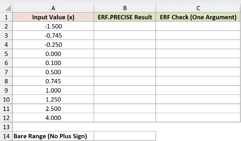
We want to calculate all eleven error-function values with one formula in B2.
Here is the formula:
=ERF.PRECISE(+A2:A12)
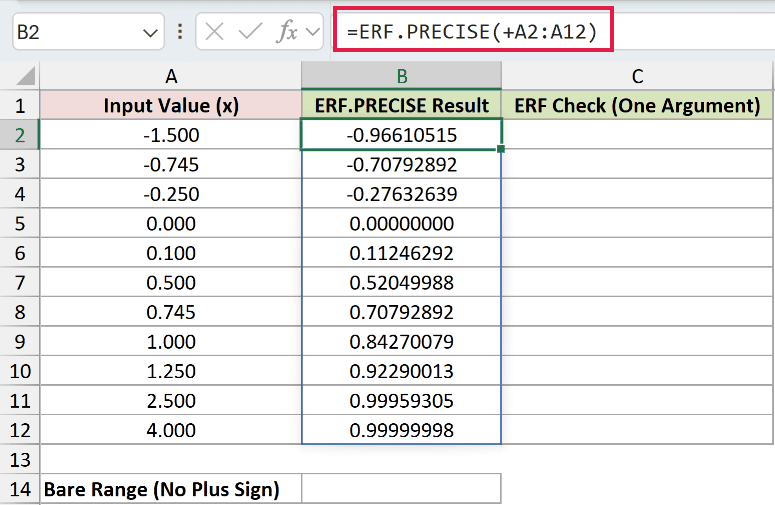
The plus sign converts the range reference into an array of values. In Excel 2021, Excel 2024, and Microsoft 365, the results spill into B2:B12.
For 0.745 in A8, the result displays as 0.70792892. For -0.745 in A3, it displays as -0.70792892. Zero returns zero.
The input 4 returns approximately 0.99999998. As positive inputs increase, the result approaches 1.
To compare the results, enter this formula in C2 and fill it down through C12:
=ERF(A2)
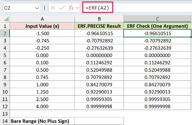
Both columns return matching values throughout. In row 2, both results display as -0.96610515 for the input -1.5.
Finally, enter the bare-range version in B14 to see how Excel handles the range without the plus sign:
=ERF.PRECISE(A2:A12)
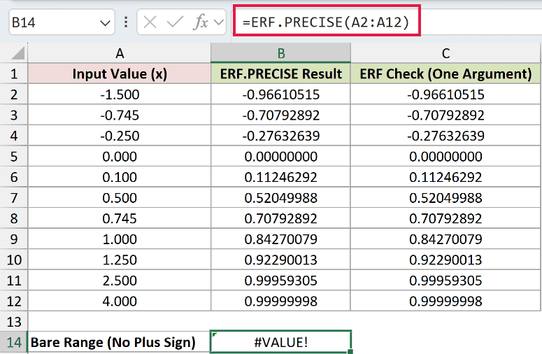
B14 returns a single #VALUE! error. Unlike the first formula, this version passes a range reference directly to ERF.PRECISE.
Pro Tip: Keep B3:B12 empty before entering the spill formula. In Excel 2019 and earlier versions that support ERF.PRECISE, use a single-cell reference and fill down instead.
Example 2: Estimate Customers per Shirt Size
Now let’s use two ERF.PRECISE calls to calculate the share between two measurement limits.
Below is the dataset with shirt sizes, chest measurement limits, an empty Share of Customers column, and the average and standard deviation in F2:G2.
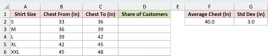
We want to estimate the customer share for each size, assuming chest measurements follow a normal distribution with mean 40 inches and standard deviation 3 inches.
Here is the formula:
=(ERF.PRECISE((C2-$F$2)/($G$2*SQRT(2)))-ERF.PRECISE((B2-$F$2)/($G$2*SQRT(2))))/2
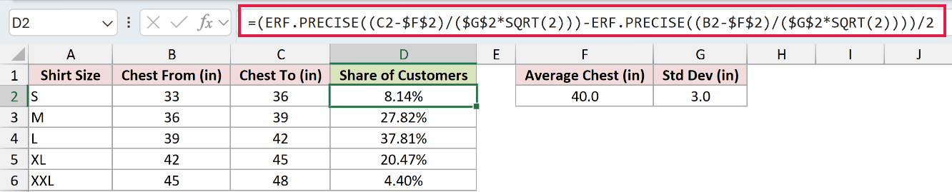
Enter the formula in D2 and fill it down through D6. Format the results as percentages with two decimal places.
How this formula works:
C2-$F$2subtracts the average chest measurement from the upper limit, 36 inches.- Dividing by
$G$2*SQRT(2)scales that difference for the error function. The second call does the same for the lower limit, 33 inches. - Subtracting the lower-limit result from the upper-limit result isolates the band. Dividing by 2 converts it into a normal-distribution probability.
- The dollar signs keep F2 and G2 fixed as you fill down.
Size S returns 8.14%. Size L, covering 39 to 42 inches, has the largest estimated share at 37.81%.
The five size bands total approximately 98.64%. The remaining customers fall below 33 inches or above 48 inches under this model.
Pro Tip: ERF.PRECISE has no second limit argument, so this band calculation needs two calls. ERF’s two-argument form can handle both scaled limits in one call.
Example 3: Calculate Readings Within Temperature Tolerance
A tolerance centered on the average lets us simplify the calculation to one call.
Below is the dataset with office zones, reading standard deviations, allowed temperature deviations, and an empty Share Within Tolerance column.
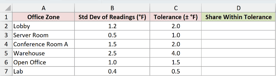
We want the estimated share within each zone’s tolerance, assuming normally distributed readings centered on the thermostat setpoint.
Here is the formula:
=ERF.PRECISE(C2/(B2*SQRT(2)))
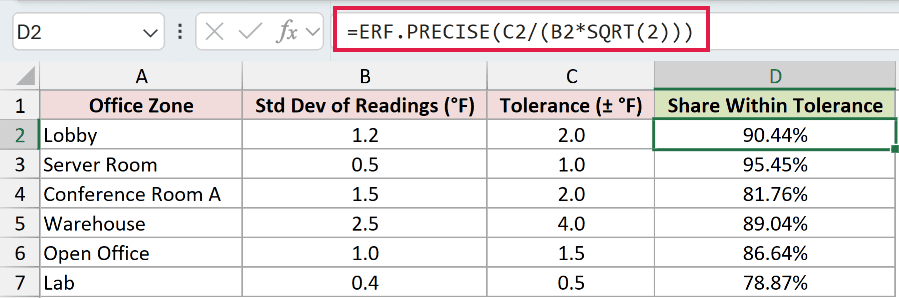
Fill the formula down from D2 through D7. Use percentage formatting with two decimal places to display the estimated shares.
How this formula works:
C2contains the allowed deviation on either side of the setpoint. For the Lobby, that is 2°F below or above it.B2contains the standard deviation, 1.2°F. Dividing the tolerance by this value expresses it in standard deviations.SQRT(2)supplies the scaling needed by the error function.- Because the limits are equally far from the mean, symmetry combines the subtraction and halving from Example 2 into one ERF.PRECISE call.
The Lobby returns 90.44%. The Server Room returns 95.45% for a tolerance of ±1°F and standard deviation of 0.5°F.
The Lab returns 78.87%. Its ±0.5°F tolerance spans fewer standard deviations than the Server Room’s tolerance, so a smaller share falls inside it.
Pro Tip: This shortcut assumes the average reading equals the setpoint. If the average drifts away from it, use separate lower and upper limits as in Example 2.
Example 4: Convert Data Usage into Percentiles
For an individual value, we can turn ERF.PRECISE into an at-or-below probability.
Below is the dataset with subscribers, monthly data usage, an empty Usage Percentile column, and the average and standard deviation in E2:F2.
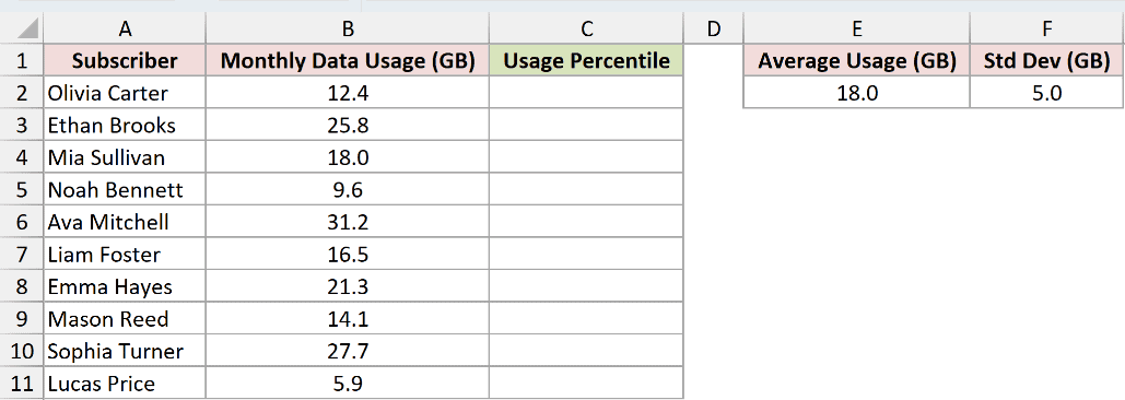
We want each subscriber’s estimated usage percentile under a normal model with mean 18 GB and standard deviation 5 GB.
Here is the formula:
=(1+ERF.PRECISE((B2-$E$2)/($F$2*SQRT(2))))/2
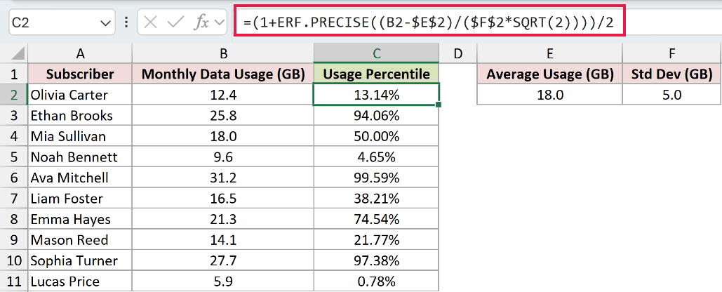
Enter the formula in C2 and fill it down through C11. Display C2:C11 as percentages, keeping two decimal places.
How this formula works:
B2-$E$2measures how far Olivia Carter’s 12.4 GB sits from the 18 GB average.- Dividing by
$F$2*SQRT(2)scales the difference using the 5 GB standard deviation. - ERF.PRECISE returns the error-function value. Adding 1 and dividing by 2 converts it into the estimated share at or below that usage.
- Absolute references keep the model’s average and standard deviation fixed when the formula is filled down.
Olivia’s result is 13.14%. Under this model, about 13.14% of subscribers use 12.4 GB or less per month.
Mia Sullivan uses exactly 18 GB, the model average. Her scaled input is zero, so the result is 50.00%, placing her at the 50th percentile.
Ava Mitchell’s 31.2 GB returns 99.59%. These percentiles describe positions in the assumed distribution, rather than ranks calculated from the ten listed subscribers.
Pro Tip: NORM.DIST with its cumulative argument set to TRUE calculates this probability directly from the usage, mean, and standard deviation. The ERF.PRECISE approach helps when adapting an existing error-function calculation.
Tips & Common Mistakes
- Use numeric inputs. A nonnumeric argument returns
#VALUE!. A bare range can also return this error, as Example 1 shows. - Keep the plus sign in the spill formula. It converts the range into values that ERF.PRECISE can process together. Clear any cells blocking the output range if you get
#SPILL!. - Distinguish the two function names. ERF.PRECISE matches one-argument ERF. Its name does not establish that it produces more accurate results.
- Keep the normal-distribution scaling. The probability examples require division by
SQRT(2)as well as the standard deviation. Use a positive standard deviation. - Check the model. The estimated shares and percentiles depend on a normal-distribution assumption and suitable mean and standard deviation values.
- Choose the right companion. ERF accepts two limits. ERFC and ERFC.PRECISE return the complementary error function, useful when working with tail calculations.
In this article, I showed you how to use ERF.PRECISE and adapt its results for normal-distribution probabilities.
I hope you found this article helpful.
Related Excel Functions / Articles:
