
The ODDLYIELD function in Excel returns the annual yield of a bond with an odd last coupon period, meaning its final interest period is shorter or longer than usual.
You supply the purchase price and bond terms, including the last coupon date before maturity. Settlement must fall after that coupon date and before maturity.
The yield reflects the price you pay as well as the remaining interest, so it can differ from the bond’s stated coupon rate.
I’ll show you how to calculate yields for a bond list, compare short and long final periods, and diagnose inputs that return errors.
ODDLYIELD Function Syntax in Excel
ODDLYIELD uses the following arguments:
=ODDLYIELD(settlement, maturity, last_interest, rate, pr, redemption, frequency, [basis])
- settlement (required): The date you buy the bond, after its last coupon date and before maturity.
- maturity (required): The date the bond is repaid.
- last_interest (required): The last coupon payment date before maturity. This marks the start of the final coupon period.
- rate (required): The annual coupon rate, entered as a percentage.
- pr (required): The purchase price per $100 of face value.
- redemption (required): The amount repaid at maturity per $100 of face value.
- frequency (required): The regular coupon schedule. Use
1for annual,2for semiannual, or4for quarterly payments. - basis (optional): The day-count convention used to measure the interest period. Omitting it uses
0.
The basis codes are:
- 0: US (NASD) 30/360.
- 1: Actual/actual.
- 2: Actual/360.
- 3: Actual/365.
- 4: European 30/360.
When to Use ODDLYIELD Function
- Calculate a yield from a quoted price when the bond is already in its final, irregular coupon period.
- Compare bonds with different final coupon dates and payment frequencies.
- Check how changes in the purchase price affect yield near maturity.
- Compare day-count conventions while holding the other bond terms fixed.
Example 1: Calculate an Odd-Last-Period Yield
Let’s start with a bond whose final interest payment falls before the next regular coupon would be due.
Below is the dataset. The card in columns A and B holds the bond’s dates, coupon rate, price, redemption, frequency, and basis, with a labelled Yield cell below.
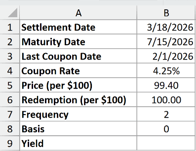
We want to calculate the annual yield from the bond terms in B1:B8.
Enter this formula in B9:
=ODDLYIELD(B1,B2,B3,B4,B5,B6,B7,B8)
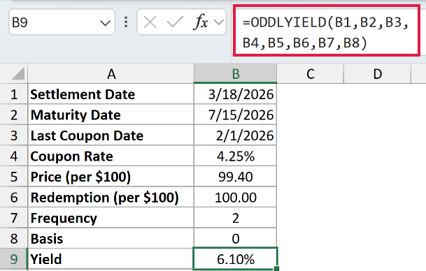
The result is 6.10%. The coupon rate is 4.25%, but the purchase price of 99.40 is below the redemption value of 100.00.
That discount contributes to the yield, along with the remaining interest payment.
The last coupon date is 2/1/2026, settlement is 3/18/2026, and maturity is 7/15/2026. Settlement falls inside the final coupon period, as required.
Pro Tip: Format the yield cell as a percentage. Keep the annual coupon rate in B4; the frequency argument tells ODDLYIELD how often coupons are scheduled.
Example 2: Calculate Yields for a Bond List
Now let’s calculate yields for bonds with different terms using a shared settlement date.
Below is the dataset. Columns A:F hold each bond’s terms, column G will hold yields, and the I:J card contains shared settlement, redemption, and basis inputs.

We want a yield for every bond using its own dates, coupon rate, price, and frequency.
Enter this formula in G2:
=ODDLYIELD($J$2,+B2:B7,+C2:C7,+D2:D7,+E2:E7,$J$3,+F2:F7,$J$4)

The formula spills its results into G2:G7. Each row uses the shared inputs in $J$2, $J$3, and $J$4.
The + before each range makes Excel pass its numeric values to ODDLYIELD. A bare range returns a single #VALUE! instead of the yields.
This spilling formula works in Excel 2021, Excel 2024, and Microsoft 365. In Excel 2019 and earlier, use individual row references and copy the formula down.
The displayed yields are:
- Ashford County School Bond: 7.28%.
- Brennan Rail Equipment Note: 4.42%.
- Dalton Power Co. Bond: 6.40%.
- Fairmont Hospital Revenue Bond: 7.08%.
- Greenway Toll Road Bond: 6.73%.
- Holloway Industrial Note: 3.24%.
Ashford’s yield exceeds its 3.90% coupon rate because the price is 99.10, below redemption. Holloway’s 101.20 price produces a yield below its 6.00% coupon rate.
Example 3: See How Price Changes Yield
A small price change can noticeably affect the yield.
Below is the dataset. Column A contains alternative purchase prices, column B will show yields, and the D:E card holds the unchanged bond terms.
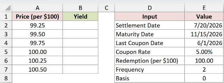
We want to compare yields while changing only the price paid for the bond.
Enter this formula in B2:
=ODDLYIELD($E$2,$E$3,$E$4,$E$5,+A2:A7,$E$6,$E$7,$E$8)
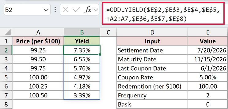
The yields spill into B2:B7. All the card references stay fixed, so each result reflects only the corresponding price in column A.
- 99.25: 7.35%.
- 99.50: 6.55%.
- 99.75: 5.76%.
- 100.00: 4.97%.
- 100.25: 4.18%.
- 100.50: 3.39%.
As the purchase price rises, the yield falls. The remaining payment is unchanged, but you pay more to receive it.
Notice that a price of 100.00 returns 4.97%, slightly below the 5.00% coupon rate. Don’t assume a price equal to redemption makes these rates identical.
Example 4: Compare Final Coupon Period Lengths
The final coupon period can be short, regular, or long, even when the other terms match.
Below is the dataset. Columns A:F list the period labels, settlement dates, maturity dates, last coupon dates, coupon rates, and prices. Column G will hold yields.

We want to compare the yields when only the maturity date changes.
Enter this formula in G2:
=ODDLYIELD(+B2:B4,+C2:C4,+D2:D4,+E2:E4,+F2:F4,100,2,0)

The final arguments are entered directly: 100 means redemption per $100 face value, 2 means semiannual coupons, and 0 selects US (NASD) 30/360.
The results spill into G2:G4:
- Short (4 months): 7.48%.
- Regular (6 months): 6.45%.
- Long (9 months): 5.85%.
Every row uses a 4.80% coupon rate and a 99.30 price. The shorter case returns the highest yield because the discount is recovered sooner.
The regular final period also returns a valid yield. ODDLYIELD doesn’t require the final period to be irregular to calculate this row.
Example 5: Check the Yield Against the Price
You can check a calculated yield by using it to recover the original bond price.
Below is the dataset. Columns A and B contain the bond terms, followed by labelled cells for Yield and Check Price.
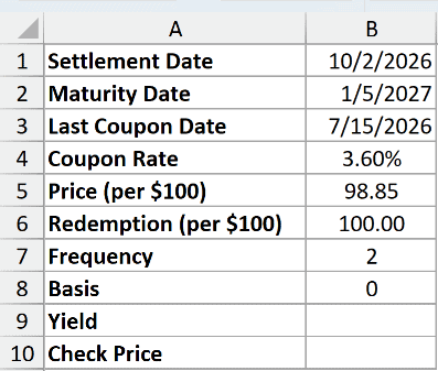
We want to calculate the yield, then confirm that it leads back to the purchase price.
First, enter the ODDLYIELD formula in B9:
=ODDLYIELD(B1,B2,B3,B4,B5,B6,B7,B8)
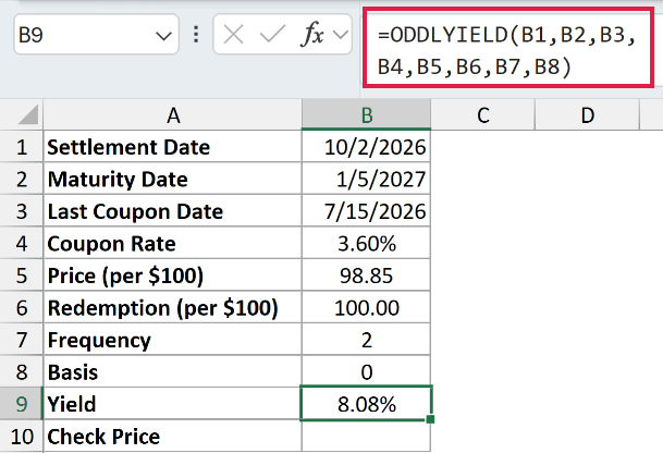
The result is 8.08%, using the 98.85 price and 3.60% coupon rate.
ODDLPRICE calculates the price of a bond with an odd last coupon period from its yield. Here, it checks the ODDLYIELD result using the same bond terms.
Enter this price-check formula in B10:
=ODDLPRICE(B1,B2,B3,B4,B9,B6,B7,B8)
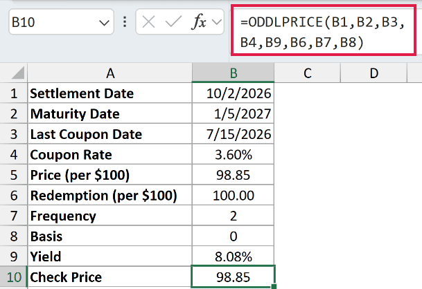
The check returns 98.85, matching the original price in B5. The formula uses the calculated yield in B9 where the price argument appeared before.
Pro Tip: Reference B9 directly when checking the price. Typing its displayed percentage into the check would use a rounded yield instead of the full calculated value.
Example 6: Compare Day-Count Bases
Let’s keep the bond fixed and change the rule used to count days.
Below is the dataset. Columns A:B list basis codes and day-count conventions, column C will hold yields, and the E:F card contains the bond terms.
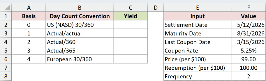
We want to see how each basis affects the yield for the same bond.
Enter this formula in C2:
=ODDLYIELD($F$2,$F$3,$F$4,$F$5,$F$6,$F$7,$F$8,+A2:A6)
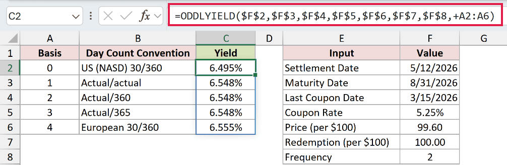
The results spill into C2:C6:
- Basis 0, US (NASD) 30/360: 6.495%.
- Basis 1, Actual/actual: 6.548%.
- Basis 2, Actual/360: 6.548%.
- Basis 3, Actual/365: 6.548%.
- Basis 4, European 30/360: 6.555%.
The actual-day conventions display the same yield in this example. A different basis code doesn’t necessarily produce a visibly different answer.
The US and European conventions do differ here. Use the convention specified for the bond when calculating its yield.
Example 7: Diagnose ODDLYIELD Errors
Finally, let’s identify the input problems that prevent a yield calculation.
Below is the dataset. Columns A:H contain scenario labels and bond inputs, including deliberate mistakes. Column I will show each result or error.
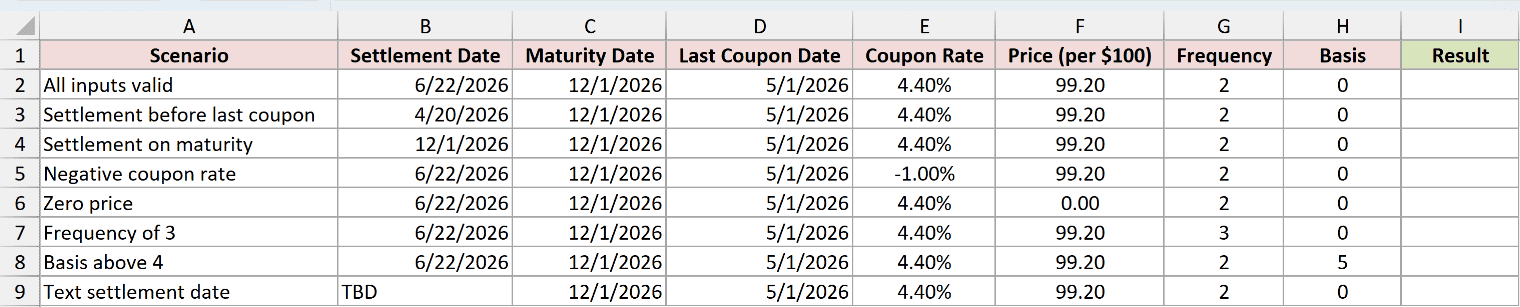
We want to calculate the valid row and identify why each remaining row fails.
Enter this formula in I2, then copy it down through I9:
=ODDLYIELD(B2,C2,D2,E2,F2,100,G2,H2)
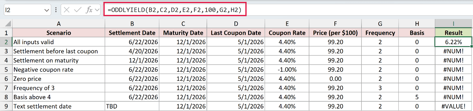
This example uses separate row formulas so each error has its own inputs to inspect. Redemption is fixed directly in the formula at 100 per $100 face value.
The valid row returns 6.22% in I2. The remaining cells deliberately show errors.
- I3,
#NUM!: Settlement is before the last coupon date. Use a settlement date inside the final coupon period. - I4,
#NUM!: Settlement equals maturity. Settlement must come before maturity. - I5,
#NUM!: The coupon rate is -1.00%. Correct the negative rate. - I6,
#NUM!: The price is 0.00. Enter a positive purchase price. - I7,
#NUM!: Frequency is 3. Select the bond’s actual annual, semiannual, or quarterly schedule. - I8,
#NUM!: Basis is 5. Use a valid day-count code. - I9,
#VALUE!: Settlement contains TBD. Replace the placeholder with a real Excel date.
Tips & Common Mistakes
- Check the date order first. Settlement must be strictly after
last_interestand strictly beforematurity. Settlement on the last coupon date also returns#NUM!. - Keep price units consistent. Both price and redemption are per $100 of face value. Don’t substitute the total cost of your bond position.
- Keep the plus signs in range formulas. ODDLYIELD needs the range values passed with
+for the spilling examples shown here. - Set the basis deliberately. Omitting it selects
0, the US (NASD) convention. That may not be the convention specified for your bond. - Use whole-number basis codes and date-only inputs. Excel truncates fractional parts of the date and basis arguments.
Before relying on a yield, confirm the last coupon date and day-count convention against the bond terms.
Other Excel articles you may also like:
