
If you want to add up the numbers sitting in a bunch of Excel cells, the tricky part is not the adding. It’s that the best way to do it changes depending on where those cells are.
Two cells sitting side by side need a different approach than eight cells scattered around the sheet. But nothing to worry about. In this article I’ll show you seven ways to add cells in Excel, and when to reach for each one.
Method #1: Using the Plus (+) Operator
This is the one everybody tries first, and for two or three cells it’s the fastest thing you can do.
Below I have a dataset with travel expenses for eight people, showing what each person spent on flights, hotels, and meals. I want to know what Priya Nair spent in total on her trip.
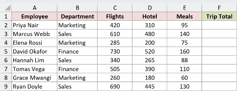
Here is the formula:
=C2+D2+E2
That gives me 825, which is 420 for flights plus 310 for the hotel plus 95 for meals.
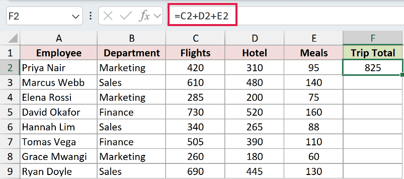
How does this formula work?
There’s not much to it. The plus sign tells Excel to take whatever number is in the first cell, add the number in the next one, and keep going.
You don’t have to type the cell addresses either. Type =, click cell C2, type +, click D2, type +, click E2, then press Enter. Excel fills in the references as you click.
The reason this method stops being useful is length. Three cells is fine. Twenty cells means typing nineteen plus signs, and if you miss one you’ll never spot it.
Note: A + formula doesn’t stretch when you insert a new row in the middle of your data. It keeps adding the exact cells you named and quietly ignores the new one.
Method #2: Using the SUM Function
Here’s another way to do the same thing, and it’s the one I’d use by default.
I’m working with the same travel expense dataset, and I still want Priya Nair’s total trip cost.
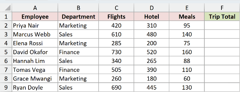
Here is the formula:
=SUM(C2:E2)
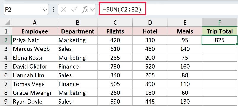
It returns 825, exactly what Method #1 gave me, with a lot less typing.
How does this formula work?
The C2:E2 bit is a range. The colon means “everything from here to there”, so C2:E2 covers C2, D2, and E2 in one go. The SUM function then adds up whatever it finds in that range.
The advantage over the plus operator shows up when the range gets long. Adding a hundred cells looks exactly the same as adding three: =SUM(C2:C101).
This also works vertically, so it’s the same formula you’d use to sum a whole column rather than a single row.
Note: SUM skips anything that isn’t a number. Blank cells and text cells don’t cause an error, they just don’t get counted.
Method #3: Using SUM With Non-Adjacent Cells
The last two methods both assumed your cells sit next to each other. Often they don’t, and adding non-adjacent cells is what this method is for.
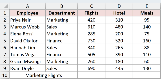
Same travel expense dataset. This time I only want the flight costs for the three people in the Marketing department, and those rows aren’t next to each other.
Priya Nair is in row 2, Elena Rossi is in row 4, and Grace Mwangi is in row 8.
Here is the formula:
=SUM(C2,C4,C8)
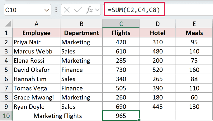
That returns 965, which is Priya’s 420 plus Elena’s 285 plus Grace’s 260.
How does this formula work?
SUM doesn’t need one tidy range. You can hand it a list of separate cells, separated by commas, and it adds all of them.
The nice part is that you don’t have to type those addresses. Type =SUM(, then hold Ctrl and click each cell you want. Excel drops in the comma for you every time you click. Release Ctrl, type the closing bracket, and press Enter.
You can mix ranges and single cells in the same formula too. Something like =SUM(C2:C4,C8,E2) is perfectly valid, so you can grab a block here and a stray cell there.
Note: SUM accepts up to 255 separate arguments. A whole range counts as just one of those, so you’ll almost never run into the limit unless you’re clicking cells one at a time.
Method #4: Using AutoSum
If you’d rather not write a formula at all, Excel has a button that writes it for you.
Same eight travel expenses, and this time I want the total of the whole Flights column in cell C10, just below the last person.
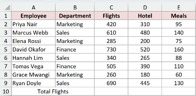
Here are the steps to add these cells with AutoSum:
- Select cell C10, the empty cell right below the flight numbers.
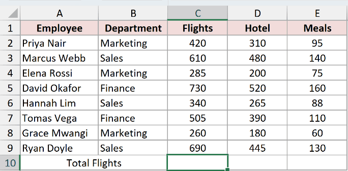
- On the Home tab, click AutoSum. Excel writes the formula and highlights the range it thinks you want.

- Check that the highlighted range is right, then press Enter.
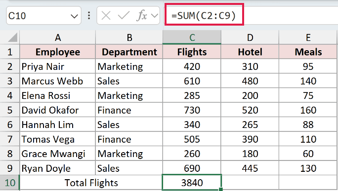
Cell C10 now shows 3840, the total of all eight flight costs.
AutoSum lives in two places on the ribbon. It’s on the Home tab and again on the Formulas tab, whichever you get to first. The keyboard shortcut is Alt + = on Windows and Shift + Cmd + T on a Mac.
All AutoSum actually does is write a SUM formula for you and pick the range it thinks you meant. Step 3 is where you get to correct it.
You can also select several empty cells at once, say C10 and D10 together, and AutoSum will fill in a separate total for each column in one go.
Note: Check the range Excel picked before you press Enter. Fixing it now takes a second, and a total that quietly covers the wrong rows is a lot harder to spot later.
Method #5: Using the Status Bar
Sometimes you don’t want a total in your sheet at all. You just want to know the number. This method gives you that without touching a single cell.
I’m back on the travel expenses, and I want to see the Flights total without adding a formula anywhere.
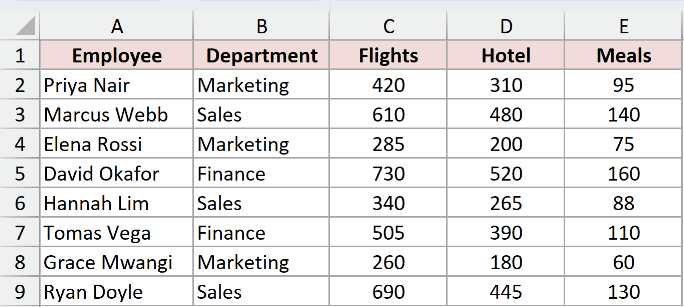
Here are the steps to add these cells using the Status Bar:
- Select the cells you want to add, in this case C2:C9.
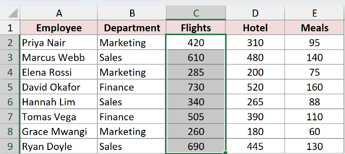
- Look at the Status Bar along the bottom right of the Excel window.
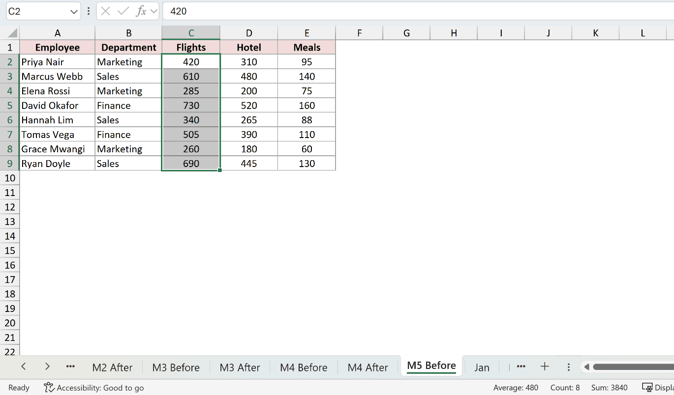
It shows Sum: 3840, along with Average: 480 and Count: 8.
This works on scattered cells too. Hold Ctrl, click whichever cells you want, and the Status Bar keeps a running total of everything you’ve selected.
Nothing gets written to the sheet and nothing gets saved. The moment you click somewhere else, the number is gone. That’s exactly what you want when you’re just sanity-checking a figure, and exactly what you don’t want when you need the total to stick around.
If you don’t see a Sum down there, right-click the Status Bar. You’ll get a list of everything it can display, and you can switch Sum back on.
Method #6: Using a 3D Reference Across Sheets
Here’s one for when your numbers aren’t all on the same sheet.
Say I’ve split the travel expenses across three sheets, one per month, named Jan, Feb, and Mar. Every sheet has the same layout, so Priya Nair’s flight cost is in cell C2 on all three. I want her flight total for the whole quarter.
Here is the formula:
=SUM(Jan:Mar!C2)
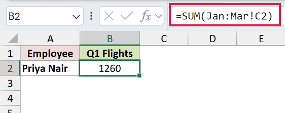
Priya’s flights were 420 in January, 385 in February, and 455 in March, so the formula returns 1260.
How does this formula work?
Jan:Mar is a 3D reference. It works like a range, except instead of running across cells it runs across sheet tabs. So Jan:Mar!C2 means “cell C2 on Jan, on Mar, and on every sheet sitting between them”.
The exclamation mark is the same one you’d use to reference a cell on another sheet normally. The only new part is putting a span of sheets in front of it instead of a single name.
You can point it at a range instead of a single cell as well. =SUM(Jan:Mar!C2:C9) would add every flight cost on all three sheets at once.
The catch is that Excel goes by tab position, not by the names you typed.
If you drag a new sheet in between Jan and Mar, its numbers get pulled into the total straight away. Drag Feb out to the end of the workbook and it drops out.
Note: If your sheet names contain spaces, Excel wraps the whole sheet range in single quotes, like =’Jan Trips:Mar Trips’!C2. Let Excel add those quotes by clicking the tabs rather than typing them yourself.
Method #7: Using Paste Special With the Add Operation
Every method so far leaves a formula behind. This one doesn’t. It changes the numbers themselves.
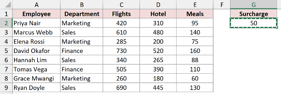
The travel expenses again. Finance has told me every flight needs a 50 fuel surcharge added on, and they want the Flights column to show the new figures directly, not a formula pointing at old ones.
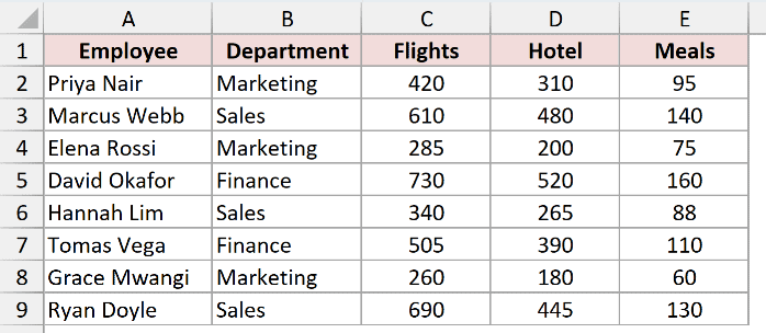
Here are the steps to add a value to these cells with Paste Special:
- Type 50 into any empty cell, press Enter, then select that cell and copy it with Ctrl + C.
- Select the cells you want to change, in this case C2:C9.
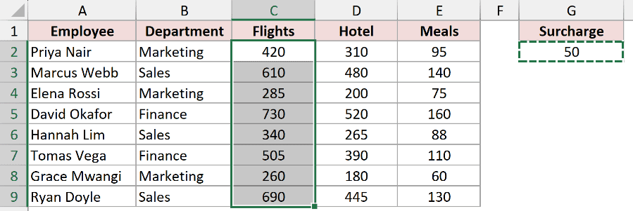
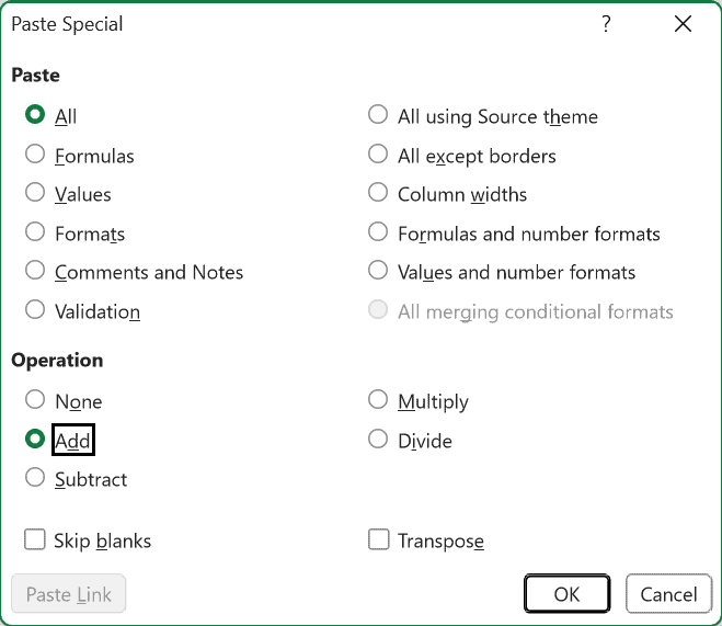
- Right-click the selection, click Paste Special, and under Operation choose Add.
- Click OK, then delete the cell where you typed the 50.
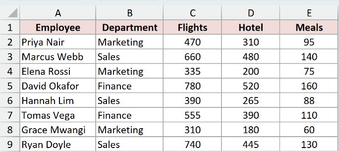
Priya’s flight cost has gone from 420 to 470, and the column total is now 4240 instead of 3840. Every one of the eight cells went up by 50.
Normally pasting replaces whatever was in a cell. Picking Add under Operation changes that. Instead of replacing, Excel takes the number you copied and adds it to whatever each cell already holds.
There’s a second use for this that saves a lot of grief. If your numbers are stuck as text and refuse to add up, copy an empty cell, select the problem range, and run Paste Special with Add.
Adding nothing forces Excel to treat every cell as a real number.
Note: This overwrites your original values, and no formula is left behind to record what happened. Make a copy of your data first if you might need the old numbers back.
Additional Notes About Adding Cells in Excel
- If SUM returns 0 but the numbers look fine, they’re text. SUM ignores text, so it adds nothing at all. The giveaway is that
=C2+C3+C4over the same cells still returns the right answer, because the plus operator converts text that looks like a number while SUM refuses to. Select the range, click the warning icon, and pick Convert to Number. That warning icon is the same green triangle you see in the corner of the cells. - SUM stays quiet about missing data. Blanks and text cells get skipped rather than flagged, so a total can look perfectly healthy while half the rows never made it in. Compare the Count in the Status Bar against how many rows you expect.
- Adding cells includes hidden and filtered rows. SUM doesn’t care what’s on screen. The SUBTOTAL function skips rows that a filter took out, whatever function number you give it. Rows you hid by hand are different, and only the 101 to 111 codes ignore those.
- Plus formulas don’t grow, SUM ranges usually do. Insert a row in the middle of your data and a
=C2+C3+C4formula carries on ignoring it, while=SUM(C2:C4)normally stretches to include it. This is the single most common reason a total silently goes wrong. - If a total refuses to update, check the calculation mode. On the Formulas tab, Calculation Options should say Automatic. Set to Manual, your totals sit there frozen until you press F9.
Frequently Asked Questions
What’s the difference between adding cells and inserting cells in Excel?
They’re two completely different jobs that share a word. Adding cells means totalling up the values inside them, which is everything this article covers.
Inserting cells means pushing new blank cells into your sheet and shifting the existing ones out of the way. If it’s blank cells you’re after, that’s the insert cell shortcut, not SUM.
Why is my cell showing the formula instead of the total?
Two usual suspects. Either Show Formulas got switched on, which you can toggle back with Ctrl + grave accent (the key just above Tab), or the cell was formatted as Text before you typed the formula.
For the second one, set the cell format back to General, then click into the cell and press Enter to re-enter the formula.
There’s more on Excel showing the formula instead of the result if neither fix does it.
How do I add only the cells that match a condition?
Use SUMIF rather than SUM. Something like =SUMIF(B2:B9,"Marketing",C2:C9) adds the flight costs, but only on the rows where the department says Marketing. It’s a cleaner answer than picking cells by hand, and it keeps working when the data changes.
Can I add cells that have numbers mixed in with text?
Not directly. A cell holding 420 USD is text as far as Excel is concerned, so SUM will skip it entirely and the plus operator will throw a #VALUE! error.
Strip the text out into its own column first, or store the number plainly and use a currency format to display the USD part.
Why is my total off by a few cents when the numbers all look right?
Your cells are probably displaying rounded values while storing longer ones. A cell showing 12.35 might really hold 12.3456.
Widen the decimals temporarily to see what’s actually in there, and wrap your values in ROUND if you need the stored numbers to match what’s on screen.
Conclusion
Seven ways to add cells, and honestly you’ll use two of them most days. SUM handles nearly everything, so if you take one thing from this, make it SUM.
The Status Bar is worth remembering for the times you want to see a number without cluttering up your sheet.
Other Excel articles you may also like:
- AutoSum in Excel
- AutoSum in Excel (Shortcut)
- SUMIFS Function in Excel
- How to Add a Total Row in Excel Table
- How to Subtract Multiple Cells from One Cell in Excel
- How to Sum Positive Numbers in Excel (Formula)
- How to Shift Cells Down in Excel (8 Easy Ways)
- How to Divide in Excel
- How to Use SUMIF Across Multiple Sheets
