How to Protect a Sheet but Allow Slicers in Excel (and Lock Their Position)

Slicers make a report easy to filter, and sheet protection stops people from typing over your numbers. Put the two together, though, and the slicer buttons usually stop responding.

That’s because Excel locks every slicer by default, just like every cell. The fix is two settings: unlock the slicer, then tell Protect Sheet which filtering to allow.

Once it works, you’ll want the slicer to stay put. Slicers move and resize as columns change, and an unlocked slicer can be dragged around even on a protected sheet.

In this article, I’ll show you how to protect a sheet with PivotTable slicers, Table slicers, and Timelines. Then I’ll cover locking slicers in place and keeping them on screen.

Protect a Sheet but Allow Slicers

The settings you need depend on what the slicer filters. Here’s how it works for a PivotTable, an Excel Table, and a Timeline.

Method #1: Using Protect Sheet With a PivotTable Slicer

This is the setup you’ll use most often, since most slicers filter a PivotTable. It’s also where one missed checkbox leaves the slicer dead.

Below I have a PivotTable on the Rental Report sheet showing bike rental revenue by station and bike type. A Station slicer and a Bike Type slicer sit next to it.

I want to lock the PivotTable so nobody can edit it, but still let people click the slicer buttons.

Here are the steps to protect the sheet and keep the slicers working:

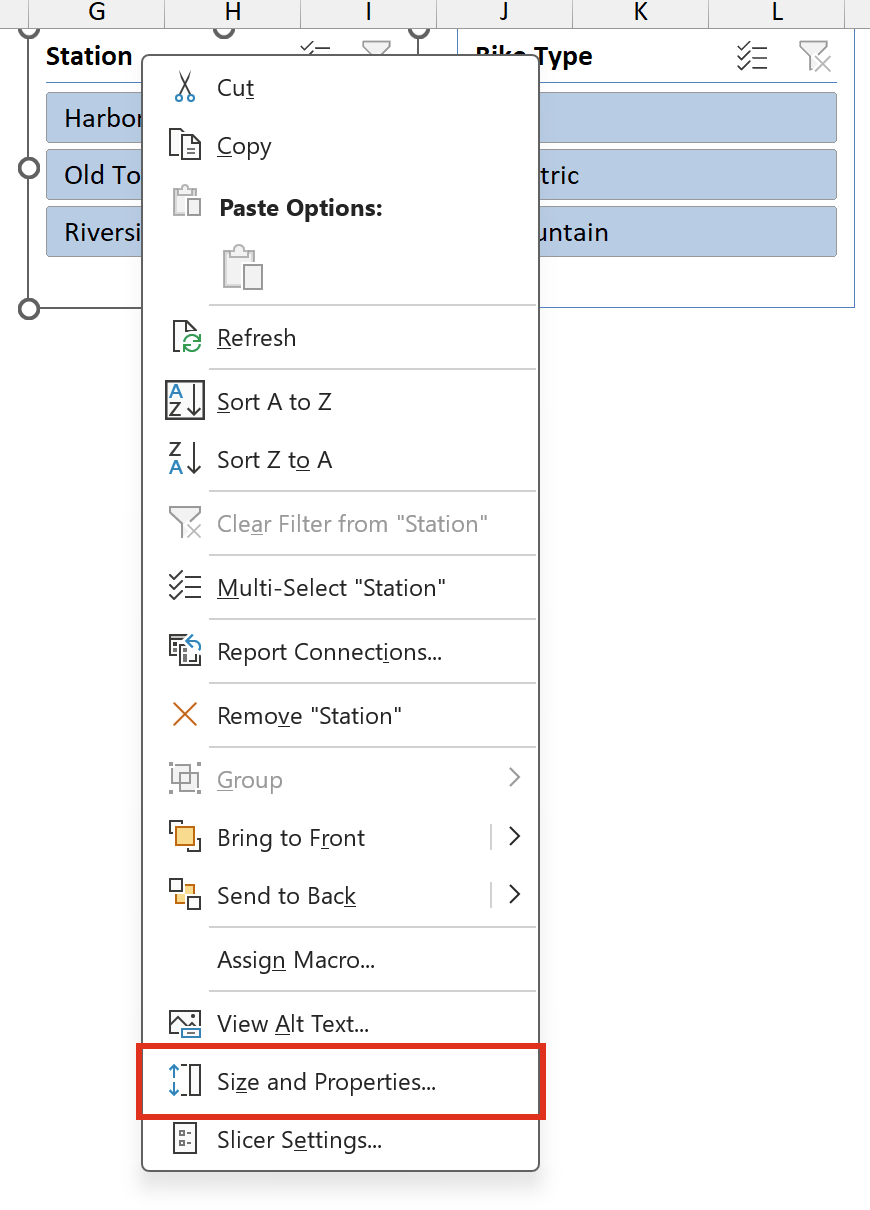
1. Right-click the Station slicer and choose Size and Properties. This opens the Format Slicer pane on the right.

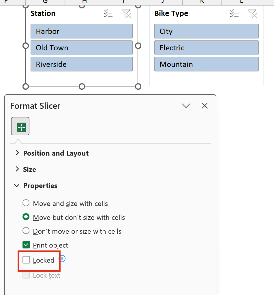
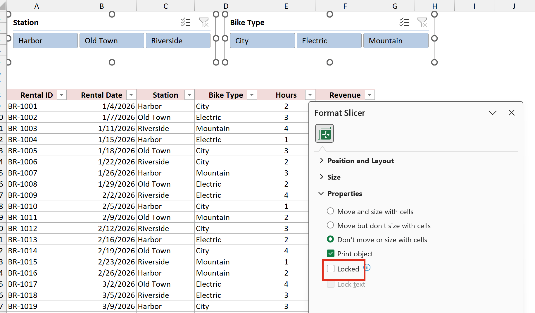
2. Expand Properties and uncheck Locked. Do the same for the Bike Type slicer.

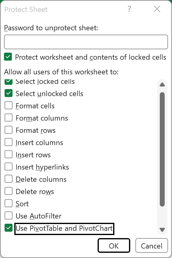
3. Go to the Review tab and click Protect Sheet. In the list of options, check Use PivotTable and PivotChart, add a password if you want one, and click OK.

The sheet is now protected, but the slicers still filter the PivotTable. Below, I clicked Harbor in the Station slicer, and the report shows only Harbor’s $272 in revenue.

If you skip step 2, the slicer stays locked and ignores your clicks. There’s no error message, which is why this one is easy to miss.

Note: You don’t need to check Edit objects for slicers to work. Some guides say you do, but I tested it and slicers filter fine without it. Leaving it unchecked also keeps people from moving or deleting the other, still-locked objects on the sheet.

Method #2: Using Protect Sheet With a Table Slicer

A slicer doesn’t have to filter a PivotTable. You can also add one to a regular Excel Table, and that kind of slicer needs a different protection option.

Below I have the bike rental data on the Rental Data sheet, set up as an Excel Table. It has a Station slicer and a Bike Type slicer above it.

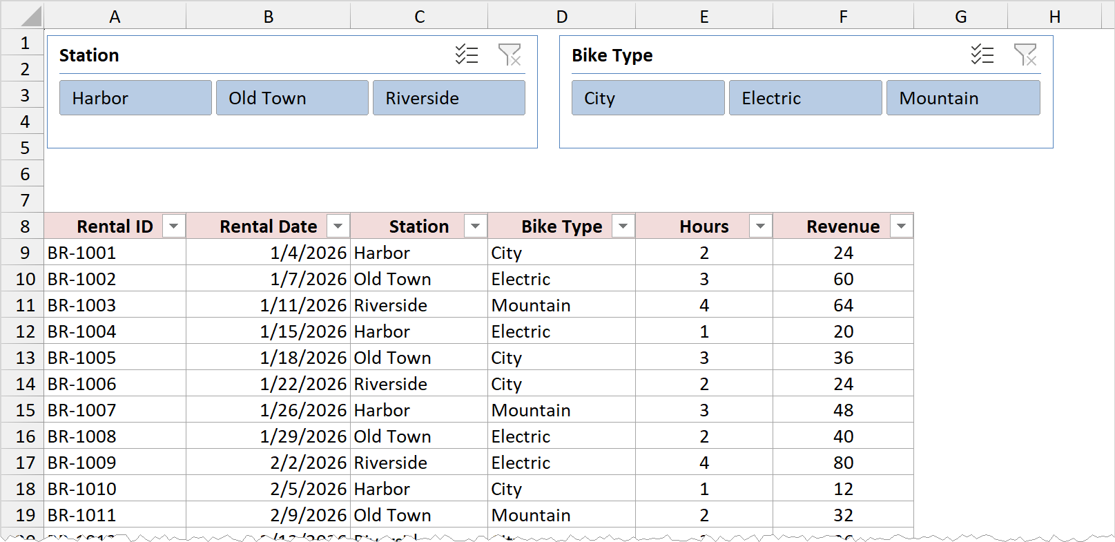
Here are the steps to protect this sheet and keep the Table slicers working:

1. Hold the Ctrl key and click both slicers to select them. Then right-click either one, choose Size and Properties, expand Properties, and uncheck Locked.

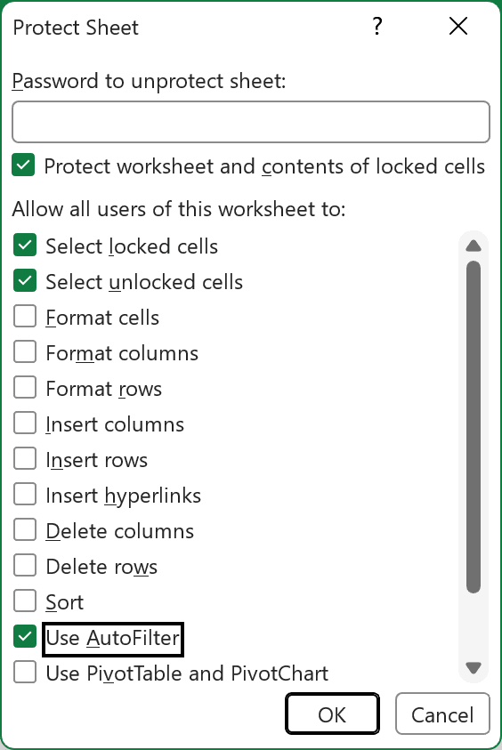
2. Go to Review and click Protect Sheet. Check Use AutoFilter, then click OK.

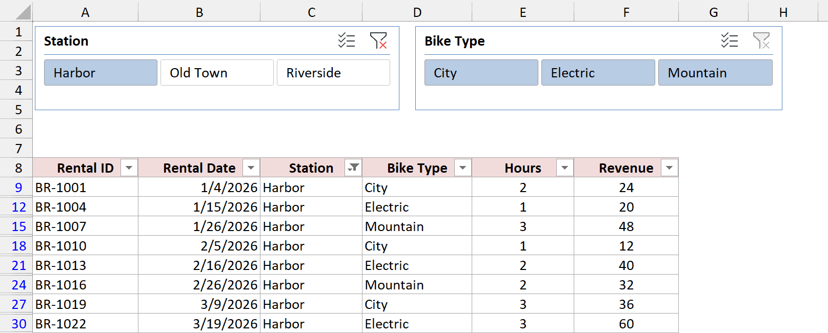
Now the slicers filter the Table even though the sheet is protected. Here, I clicked Harbor, and the Table shows only the eight Harbor rentals.

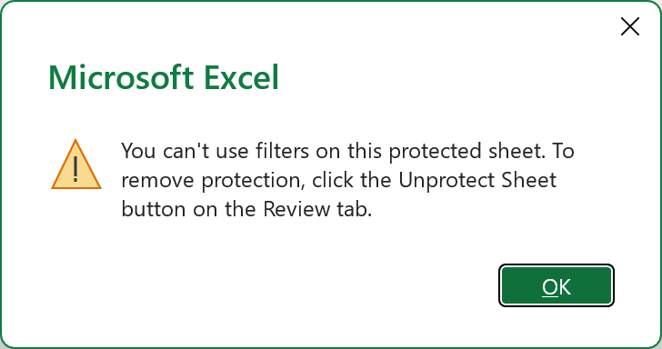
If you forget Use AutoFilter, clicking a Table slicer shows a message saying you can’t use filters on this protected sheet.

Note: If the same sheet has a Table slicer and a PivotTable slicer, check both Use AutoFilter and Use PivotTable and PivotChart.

Method #3: Using the Same Settings for a Timeline

A Timeline is a slicer built for dates. You click months, quarters, or years instead of buttons, and it needs the same two settings as a PivotTable slicer.

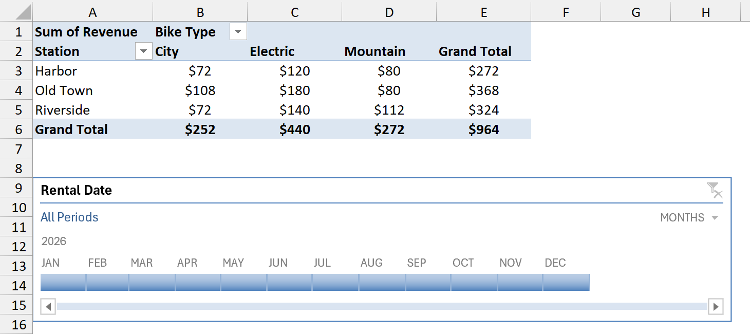
Below I have the same revenue PivotTable with a Rental Date Timeline under it.

Here are the steps to protect the sheet and keep the Timeline working:

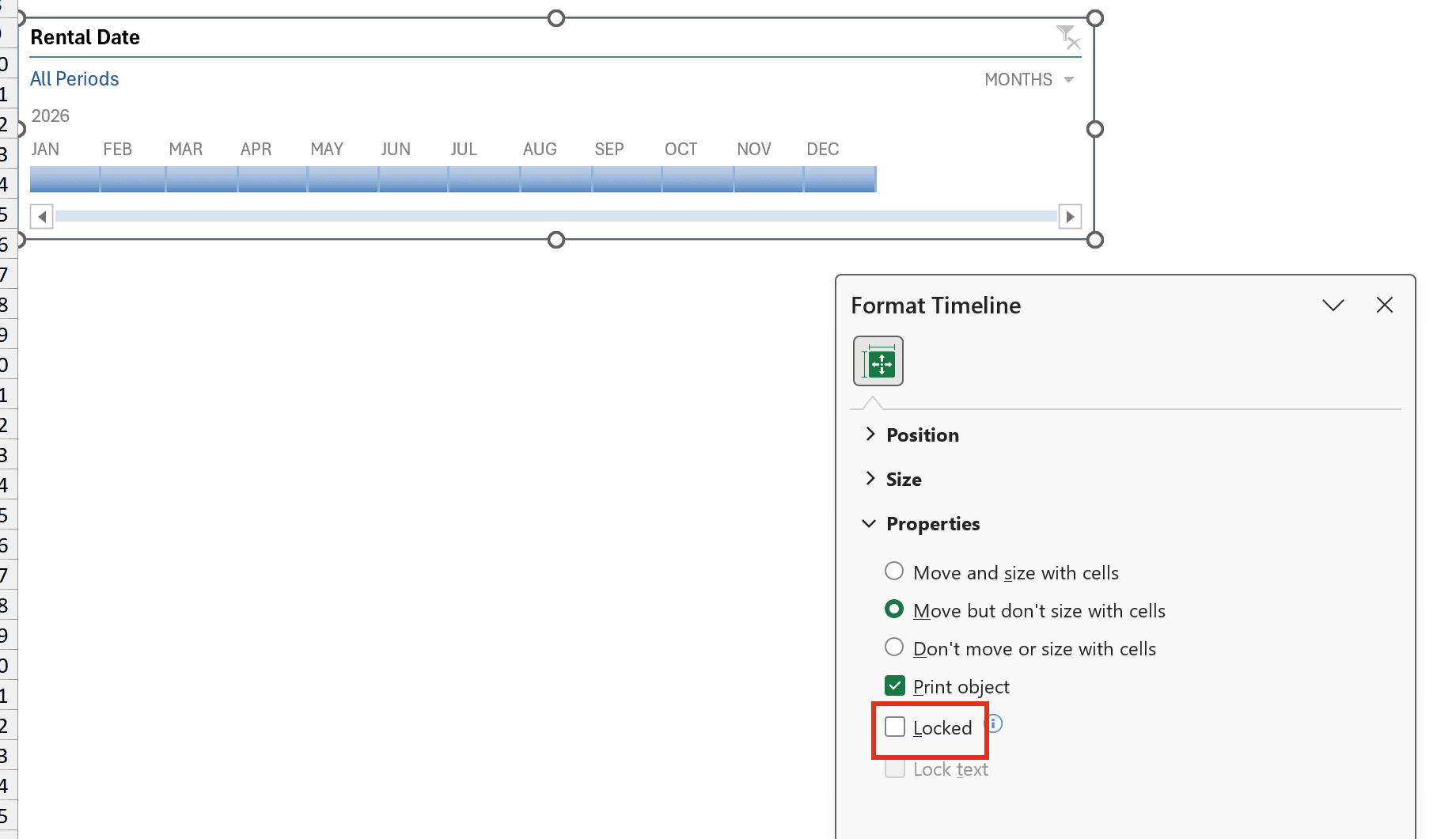
1. Right-click the Timeline and choose Size and Properties. In the Format Timeline pane, expand Properties and uncheck Locked.

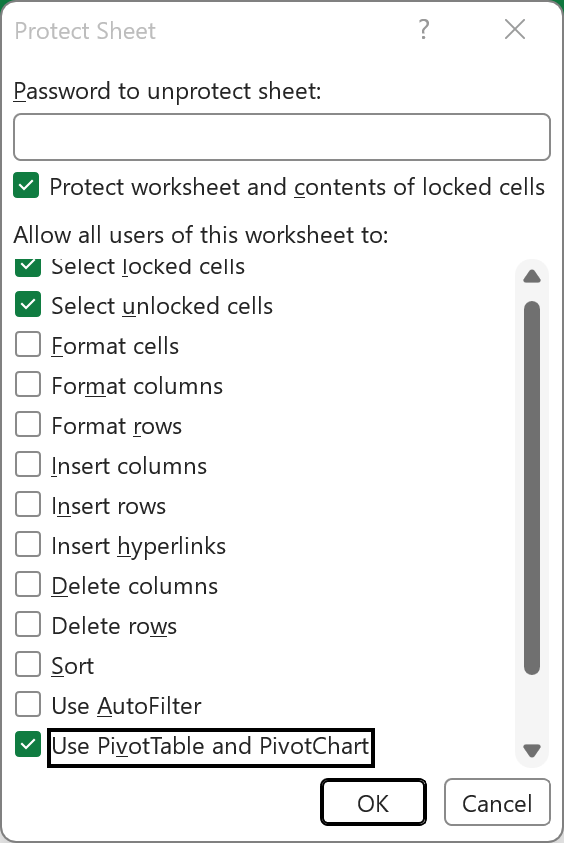
2. Go to Review, click Protect Sheet, check Use PivotTable and PivotChart, and click OK.

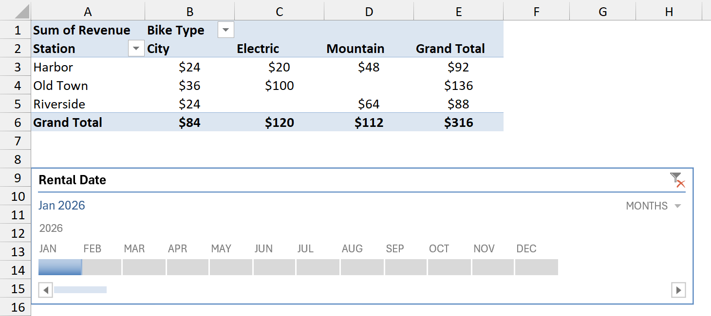
The Timeline now filters the PivotTable on the protected sheet. Below, I clicked January, and the report shows January’s $316 in revenue.

A regular slicer on a date field follows Method #1 exactly. It’s still a slicer, so it needs Locked turned off and Use PivotTable and PivotChart checked.

Lock a Slicer’s Position

A working slicer can still end up in the wrong place. It can be dragged, shift when columns change, or stretch with the cells under it. Here’s how to stop each one.

Method #4: Using Disable Resizing and Moving (Recommended)

Unlocking a slicer has a side effect. It also lets anyone drag the slicer around or resize it, even on a protected sheet. This setting stops that.

Below I have the same PivotTable report with its Station and Bike Type slicers.

Here are the steps to lock the slicer’s size and position:

1. Select the slicers (hold Ctrl to pick more than one), right-click, and choose Size and Properties. Expand Position and Layout and check Disable resizing and moving.

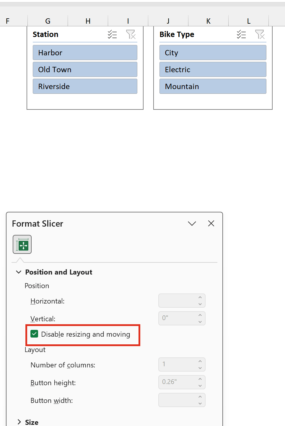
Now the slicers can’t be dragged or resized, but their buttons still work. This setting holds even without sheet protection, so you can use it on any report.

A Timeline has the same checkbox. You’ll find it under Position in the Format Timeline pane.

Note: This setting doesn’t stop someone from deleting a slicer. An unlocked slicer can still be deleted on a protected sheet, so keep a copy of the file if other people edit it.

Method #5: Using Don’t Move or Size With Cells

By default, a PivotTable slicer moves with the cells under it, but doesn’t resize. So when you insert a column or widen one to its left, the slicer slides over.

Below I have the same report, with the slicers to the right of the PivotTable.

Here are the steps to make the slicer ignore changes to the cells under it:

1. Right-click the slicer, choose Size and Properties, expand Properties, and select Don’t move or size with cells.

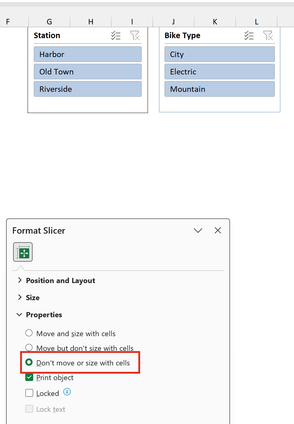
The slicer now stays where it is when you insert, delete, or resize the columns and rows around it.

This option also fixes a slicer that keeps changing size. That happens when it’s set to <strong>Move and size with cells</strong>, so it stretches whenever a column under it gets wider.

Method #6: Turning Off Autofit Column Widths on Update

Sometimes a slicer moves every time you click it, even though nobody touched the columns. The PivotTable is what’s moving it.

Below I have the report with two slicers placed to the right of the PivotTable. I widened the PivotTable’s columns a bit to make it easier to read.

When I clicked Electric in the Bike Type slicer, the PivotTable dropped two columns and shrank the rest back to fit. The slicers moved left along with those columns.

A PivotTable resizes its columns every time it updates, and filtering counts as an update. You can switch that off.

Here are the steps to lock the PivotTable column widths:

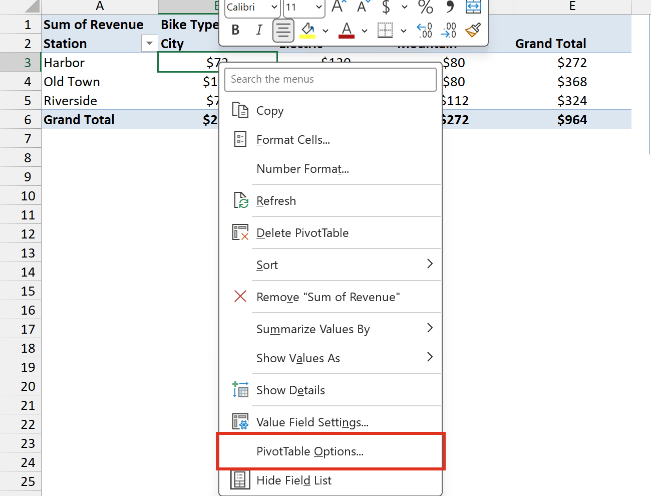
1. Right-click any cell in the PivotTable and choose PivotTable Options.

2. On the Layout & Format tab, uncheck Autofit column widths on update and click OK.

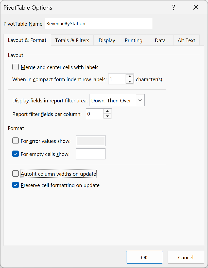
Now the column widths stay fixed when you filter, so the slicers stay put. Set the widths you want first, since Excel won’t adjust them for you anymore.

Method #5 on its own also stops the drift, because the slicer ignores the columns. I use both, so the PivotTable doesn’t jump around either.

Keep a Slicer on Screen When Scrolling

A slicer scrolls out of view with the rows under it, like any other object. Excel has no “always on top” option for slicers, but Freeze Panes gets you there.

Method #7: Using Freeze Panes

The trick is to put the slicers above your data, then freeze the rows they sit in. Frozen rows never scroll, so the slicers stay visible.

Below I have the rental Table on the Rental Data sheet, with the slicers in rows 1 to 7 and the Table’s headers in row 8.

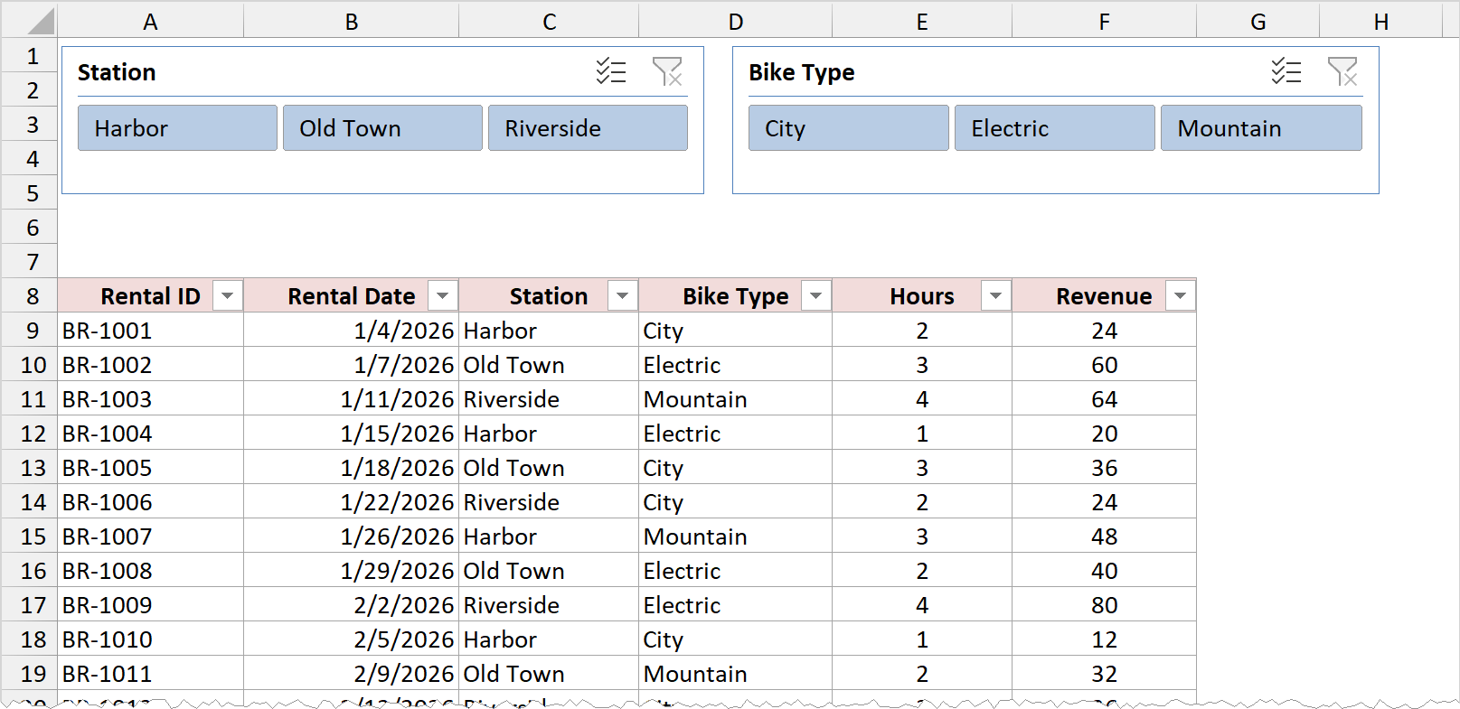
Here are the steps to keep the slicers on screen:

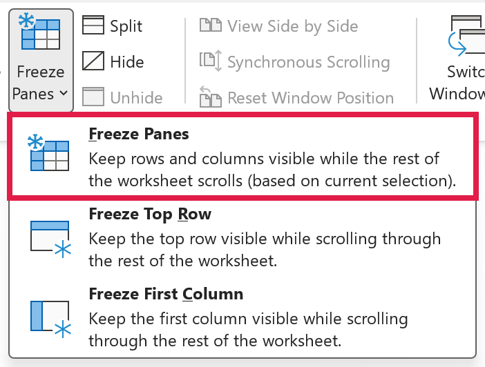
1. Select cell A9, the first cell below the headers. Then go to the View tab, click Freeze Panes, and choose Freeze Panes.

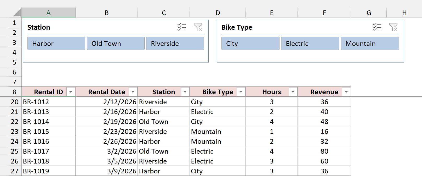
Rows 1 to 8 are now frozen. When you scroll down, the slicers and the headers stay at the top while the rentals scroll underneath.

Frozen panes stay in place after you protect the sheet, so you can combine this with Method #2. I’d set up the freeze first, then protect.

Protect the Workbook Structure

Protecting a sheet doesn’t stop anyone from deleting it, renaming it, or adding new sheets. That’s a separate, workbook-level setting.

Method #8: Using Protect Workbook

Workbook protection locks the sheets themselves in place. It doesn’t touch what’s on them, so your slicers keep working as before.

Below I have the finished Rental Report sheet, with the sheet protected and its slicers locked in place.

Here are the steps to protect the workbook structure:

1. Go to the Review tab and click Protect Workbook. Make sure Structure is checked, add a password if you want one, and click OK.

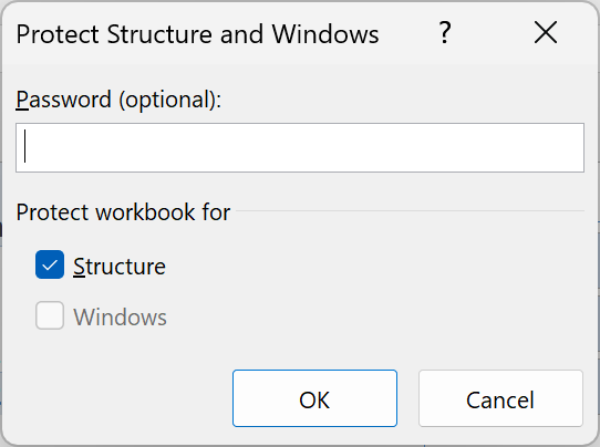
Now nobody can add, delete, rename, move, or hide sheets. Combined with sheet protection, the report is locked down, but the slicers still filter it.

Additional Notes About Protecting a Sheet With Slicers in Excel

• Every new slicer starts out locked. If you add a slicer later, unprotect the sheet, unlock the new slicer, and protect the sheet again.
• A password is optional. Without one, anyone can click Unprotect Sheet on the Review tab. With one, write it down, because Excel can’t recover a lost sheet password.
• The example file has all of this set up. Both sheets are protected with no password, so click Unprotect Sheet on the Review tab to see or change the settings.

Frequently Asked Questions

Here are some common questions about using slicers on a protected sheet.

Why doesn’t my slicer work after I protect the sheet?

Either the slicer is still locked, or Protect Sheet is missing an option. Unlock the slicer, then check Use PivotTable and PivotChart (or Use AutoFilter for a Table slicer).

Can I protect a sheet with a password and still use slicers?

Yes. The password only controls who can unprotect the sheet. It doesn’t change how the slicers behave, as long as they’re unlocked and the right option is checked.

Can people delete a slicer on a protected sheet?

Yes, if the slicer is unlocked. Unlocking it is what lets people click it, and it also lets them delete it. Disable resizing and moving doesn’t prevent that.

Why does my slicer keep changing size?

It’s set to Move and size with cells, so it changes size along with the columns and rows under it. Switch it to Don’t move or size with cells.

Conclusion

To use slicers on a protected sheet, unlock each slicer and check the matching Protect Sheet option: Use PivotTable and PivotChart for PivotTables and Timelines, Use AutoFilter for Tables.

After that, I’d turn on Disable resizing and moving for every slicer. Add Don’t move or size with cells and Freeze Panes when your layout needs them.

I hope you found this article helpful.

Other Excel articles you may also like:

• Slicer Not Working or Greyed Out in Excel (How to Fix It)
• Slicers vs Filters in Excel (Differences and When to Use Each)
• How to Create an Interactive Dashboard in Excel (With Slicers)
• Remove Old Items or Blanks From a Slicer in Excel
• How to Connect Slicer to Multiple Pivot Tables
• Pivot Table Not Refreshing – How to Fix?
• How to Lock Columns in Excel
• Change Slicer Font Size and Color
• Single-Select Slicer in Excel