How to Make a Slicer Drop-Down List in Excel

A slicer in Excel lets you filter a PivotTable with one click. But with a lot of items, it becomes a tall stack of buttons that crowds your report.

A drop-down list would fit the same choices into a single cell. The catch is that Excel has no setting to convert a slicer to a drop-down.

In this article, I’ll show you three workarounds: a report filter that works as a real drop-down, a compact one-row slicer, and a formula drop-down built with FILTER.

Method #1: Using a Report Filter Connected to the Slicer

This is the method I’d use in most reports. It gives you a real drop-down, needs no formulas or macros, and keeps every PivotTable in sync.

It works because a PivotTable’s report filter and a slicer on the same field share the same filter. Change one, and Excel updates the other.

Below I have two PivotTables built from a bookstore chain’s sales. The left one shows books and revenue by category, and the right one shows them by format.

The Branch slicer is connected to both PivotTables, so clicking a city filters both reports.

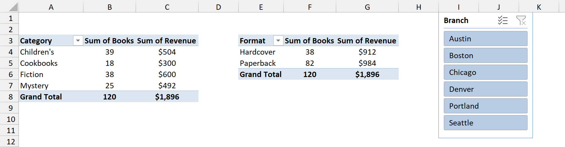
I want to replace that slicer with a drop-down that still filters both PivotTables.

Here are the steps to do this:

1. Click any cell in the Category PivotTable. In the PivotTable Fields pane, drag the Branch field into the Filters area.

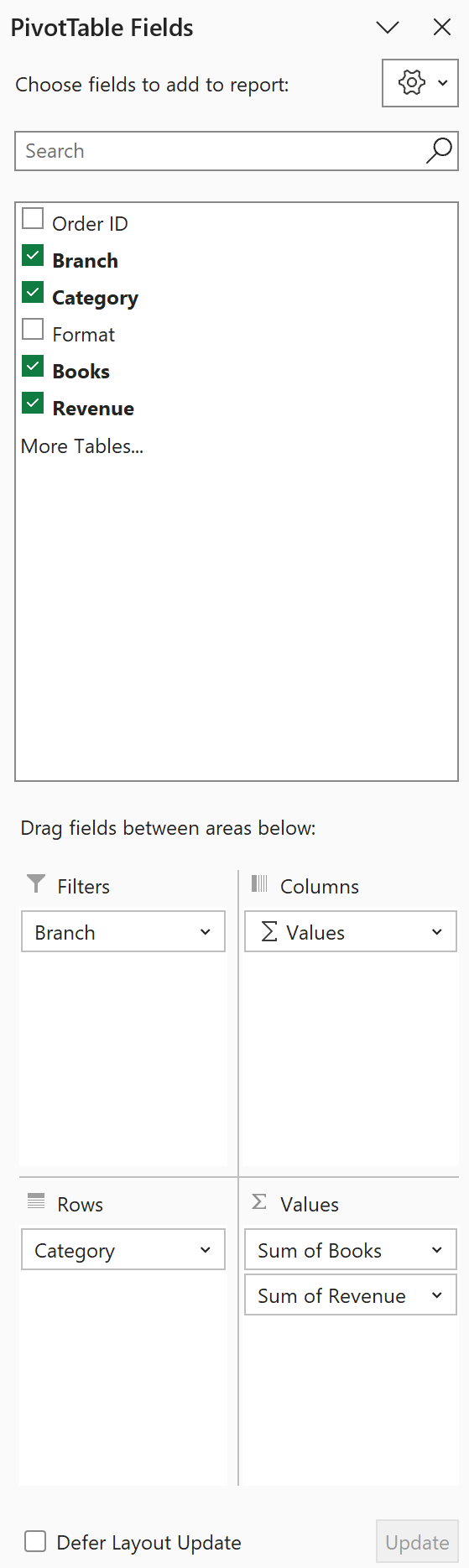
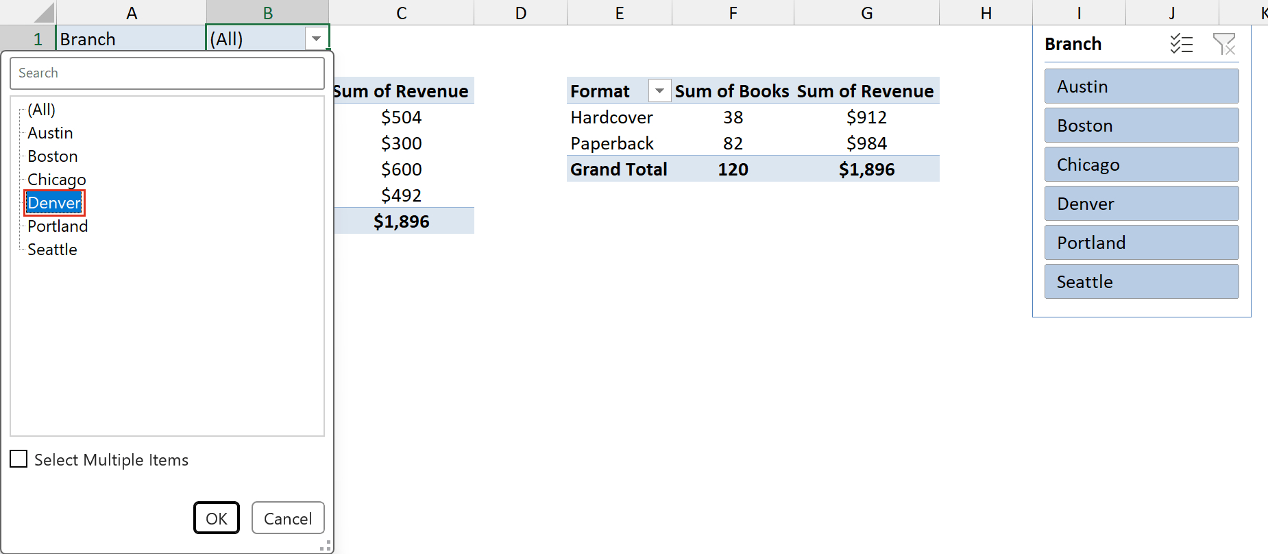
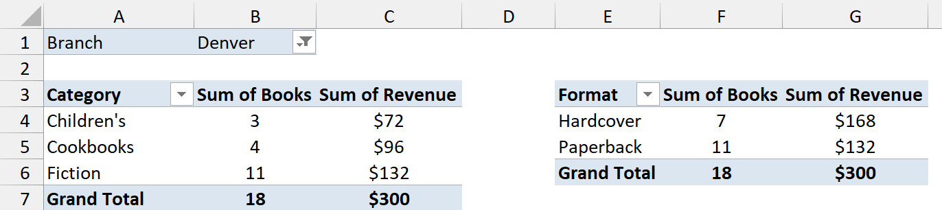
A Branch filter now sits above the PivotTable, in cells A1:B1. It shows (All) because nothing is filtered yet.

2. Click the drop-down arrow in cell B1, select Denver, and click OK.

The slicer jumps to Denver, and both PivotTables now show only Denver’s sales. That’s 18 books and $300 in revenue.

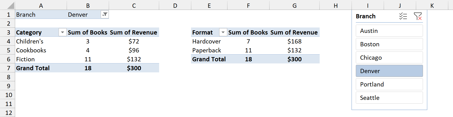
It works the other way too. Click a city on the slicer, and cell B1 changes to match.

Once the drop-down works, you don’t need to see the slicer anymore. You can hide it.

3. Press Alt + F10 to open the Selection Pane, then click the eye icon next to the Branch slicer.

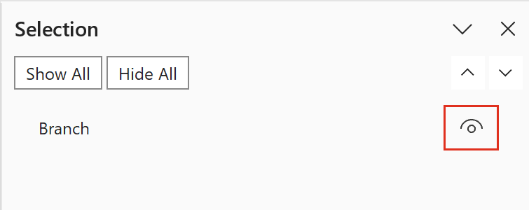
The slicer disappears, but the drop-down in B1 still filters both PivotTables.

Note: Hide the slicer, but don’t delete it. The slicer is what links the two PivotTables. If you delete it, the drop-down only filters the PivotTable it sits on.

If you only have one PivotTable, you can skip the slicer entirely. Drag the field into the Filters area, and that report filter is your drop-down.

Method #2: Using a Compact One-Row Slicer

If you like slicer buttons but want them smaller, put them in a single row. It isn’t a drop-down, but it’s nearly as slim.

Below I have a PivotTable that shows books and revenue by category, with a Branch slicer next to it. The slicer is set to Denver.

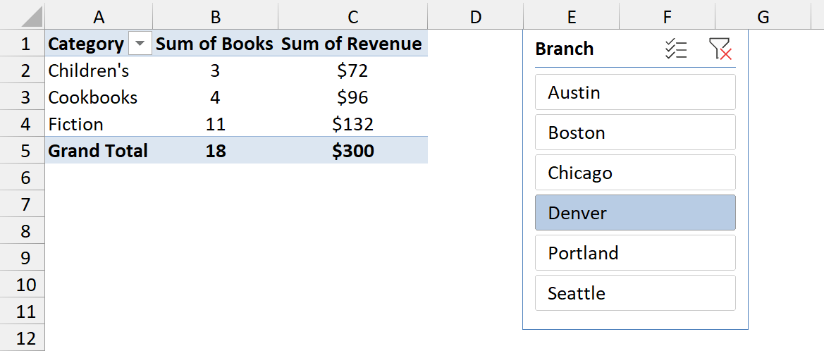
By default, a slicer shows its buttons in one tall column with a header on top. I’ll remove the header and put all six buttons side by side.

Here are the steps to make the slicer compact:

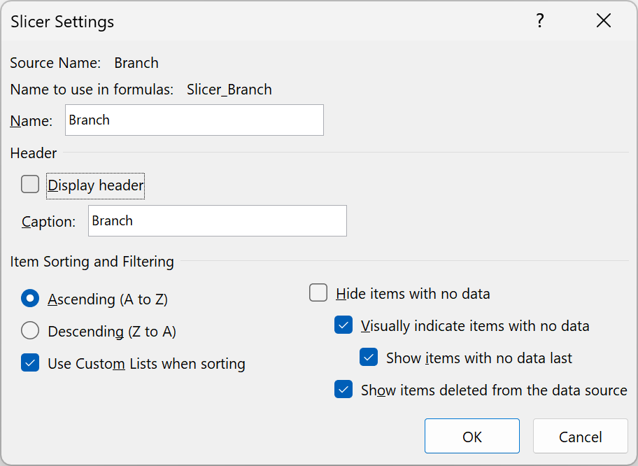
1. Right-click the slicer and choose Slicer Settings. Uncheck Display header, then click OK.

2. With the slicer selected, go to the Slicer tab. In the Buttons group, set Columns to 6 and Width to 1″. In the Size group, set Height to 0.5″.

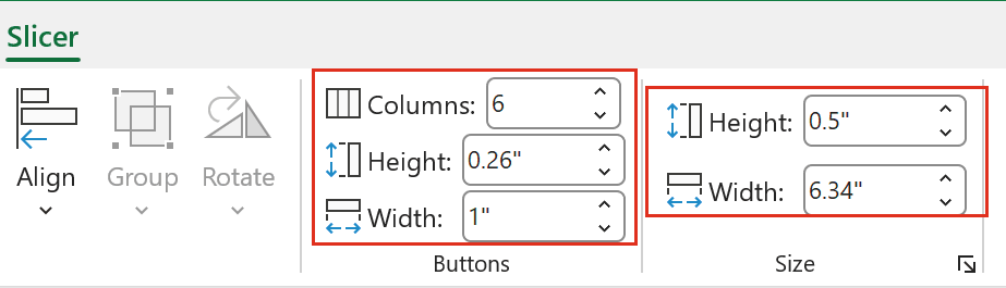
The slicer widens on its own to fit six 1-inch buttons, and it’s now a single strip you can park above the PivotTable.

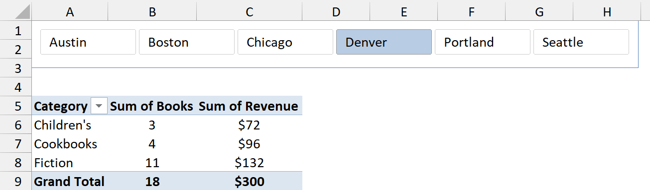
Set Columns to the number of items in your field. If there are too many to fit in one row, use the drop-down from Method #1 instead.

Note: With the header gone, the Clear Filter button goes too. To clear the slicer, select it and press Alt + C.

Method #3: Using a Data Validation Drop-Down and FILTER

If you don’t need a PivotTable at all, you can build the drop-down with a formula.

This method needs Microsoft 365, Excel 2021, or Excel 2024, because it uses dynamic array functions.

You’ll use a data validation drop-down list to pick a branch, and the FILTER function to return that branch’s orders.

Below I have the bookstore sales data in an Excel Table named BookSales. It has the order ID, branch, category, format, number of books, and revenue for each order.

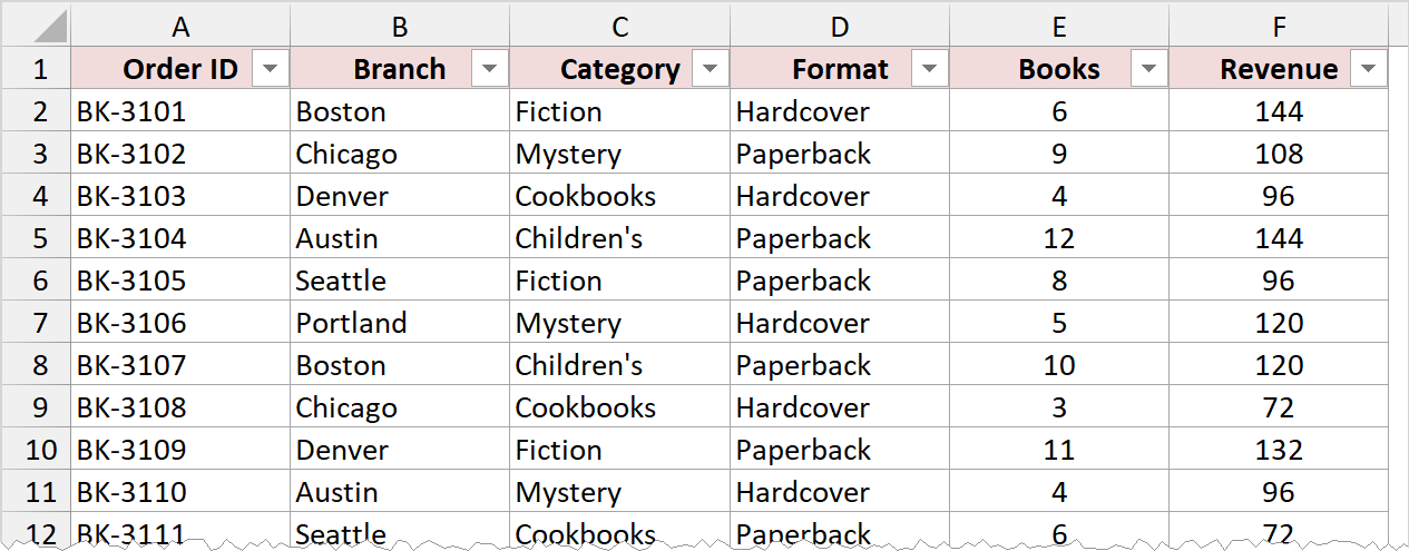
On a separate sheet, I want to pick a branch in cell B1 and see only that branch’s orders below it.

First, I need a list of branches for the drop-down. This formula in cell H2 returns each branch once, sorted A to Z:

=SORT(UNIQUE(BookSales[Branch]))

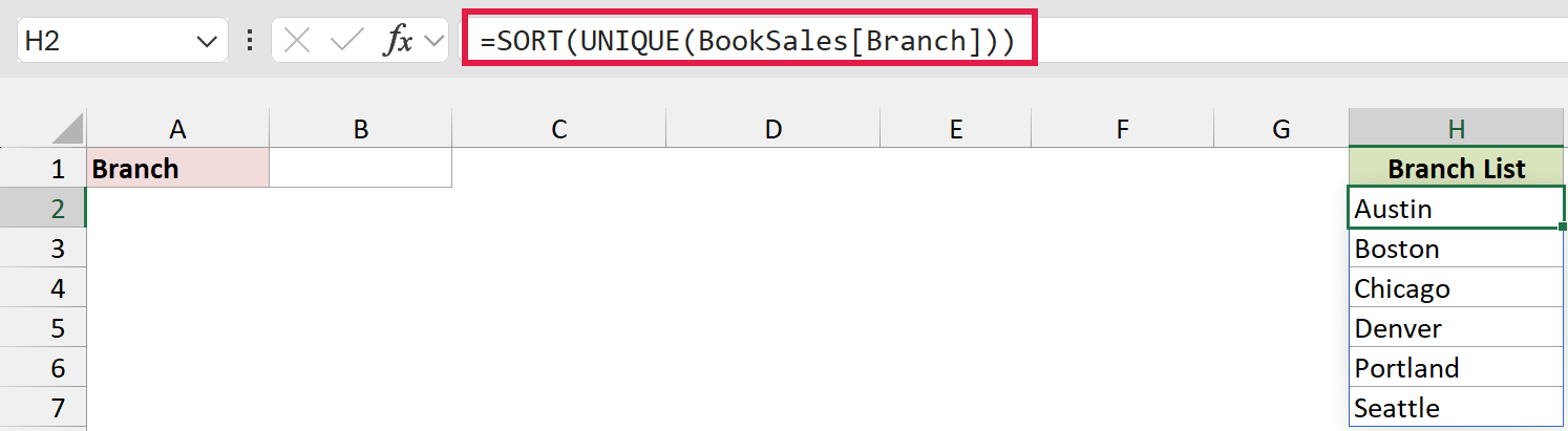
The formula spills down to H7. If you add a new branch to the table, it shows up in this list automatically.

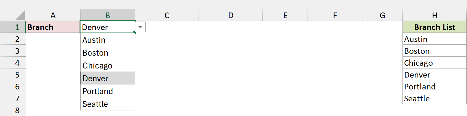
Now I’ll turn cell B1 into a drop-down that reads from this list.

Here are the steps:

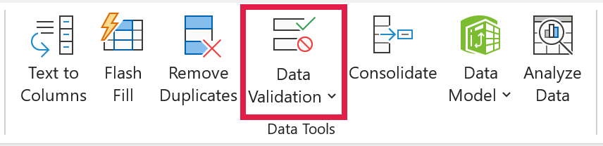
1. Select cell B1, go to the Data tab, and click Data Validation.

2. In the Allow drop-down, choose List. In the Source box, type =$H$2# and click OK.

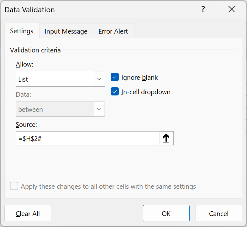
The # after $H$2 tells Excel to use the whole spill range, however many branches the formula returns.

3. Click the arrow next to cell B1 and select Denver.

Finally, I’ve typed the table’s column headers in A3:F3. Here is the formula in cell A4 that returns the matching orders:

=FILTER(BookSales,BookSales[Branch]=B1)

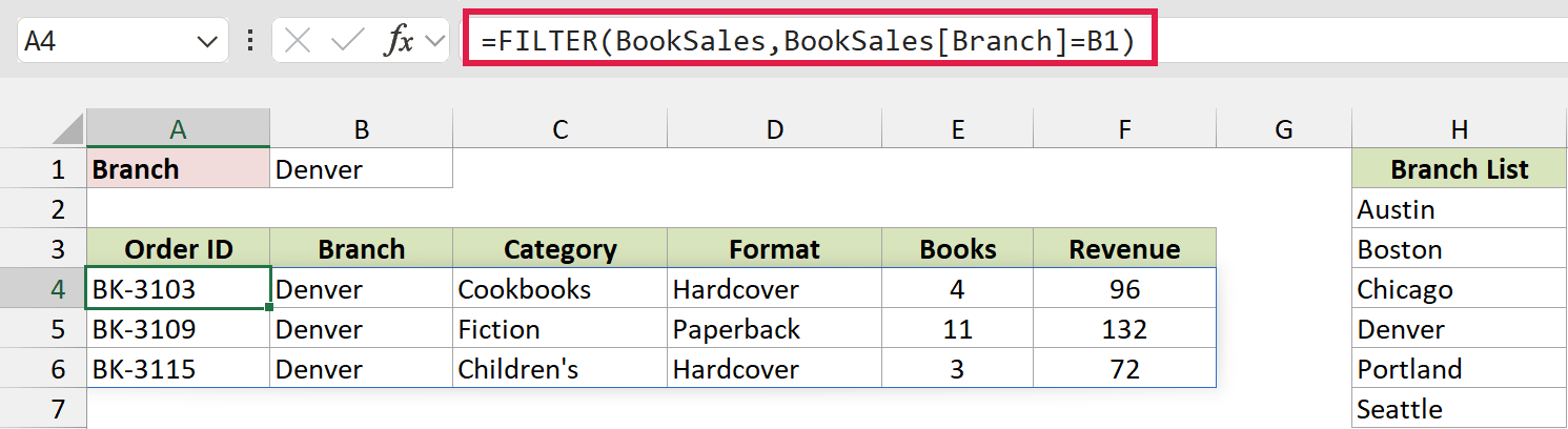
It returns Denver’s three orders. Pick another branch in B1, and the results update right away.

How does this formula work?

FILTER takes the whole BookSales table as the data to return. The second part, BookSales[Branch]=B1, checks each row’s branch against the one you picked.

FILTER keeps only the rows where that check is TRUE and spills them below the formula.

Note: If you add a new order to the BookSales table, FILTER picks it up automatically. There’s nothing to refresh.

Additional Notes About Making a Slicer Drop-Down List in Excel

• Methods #1 and #2 work with PivotTables. Method #3 works straight from a table, so use it when there’s no PivotTable involved.
• PivotTables don’t refresh on their own. When your source data changes, go to the Data tab and click Refresh All, or the Method #1 drop-down won’t list new branches.
• The shortcuts in this article (Alt + F10 and Alt + C) are for Excel on Windows.

Frequently Asked Questions

Here are some questions people often ask about slicer drop-downs.

Can I convert a slicer into a drop-down list in Excel?

No. Excel has no setting that turns a slicer into a drop-down. A report filter connected to the slicer (Method #1) is the closest built-in option.

Can the report filter drop-down select more than one item?

Yes. Check Select Multiple Items at the bottom of the drop-down, then tick the items you want. The cell shows (Multiple Items), and the slicer and PivotTables follow.

Does Method #1 work with a slicer on an Excel Table?

No. Only PivotTables have a Filters area, so the report filter trick needs a PivotTable. For data in an Excel Table, use the data validation and FILTER method instead.

Can I put the drop-down on a different sheet from the PivotTables?

Yes. Put the report filter on a PivotTable on that sheet, and connect the slicer to it and your other PivotTables. The drop-down then controls them all.

Conclusion

Excel can’t turn a slicer into a drop-down, but you can get very close.

In this article, I showed you a report filter connected to the slicer, a compact one-row slicer, and a data validation drop-down with FILTER.

For most PivotTable reports, I’d go with the report filter, since it’s a real drop-down that keeps every connected PivotTable in sync.

I hope you found this article helpful.

Other Excel articles you may also like:

• How to Show the Slicer Selection in a Cell in Excel
• How to Create an Interactive Dashboard in Excel (With Slicers)
• Slicer Not Working or Greyed Out in Excel (How to Fix It)
• Remove Old Items or Blanks From a Slicer in Excel
• How to Lock a Pivot Table in Excel
• Limit a Slicer to One Selection
• Add a Search Box to a Slicer
• Format Slicers in Excel