If you want to find the position of a value inside a list or a row of headers, the MATCH function in Excel is built for exactly that.
It returns the position number (1, 2, 3, and so on), not the value itself, which is why it pairs so naturally with INDEX for two-way lookups. In Excel 365, you can also feed MATCH an array of lookup values and the positions will spill into the cells below.
MATCH Function Syntax
Here is the syntax of the MATCH function:
=MATCH(lookup_value, lookup_array, [match_type])
- lookup_value – The value you want to find. Can be a number, text, a logical value, or a cell reference.
- lookup_array – The single row or column of cells you want to search.
- match_type – Optional. Controls how the match happens. Use 0 for an exact match (the most common case), 1 for the largest value less than or equal to lookup_value (array must be sorted ascending), or -1 for the smallest value greater than or equal to lookup_value (array must be sorted descending). Defaults to 1 if you leave it out, which is a common source of bugs, so it’s worth always passing 0 unless you specifically need a range match.
When to Use the MATCH Function in Excel
Use this function when you need to:
- Find where a value sits in a column or row so you can use that position somewhere else.
- Pair with INDEX for a flexible two-way lookup that works in any direction.
- Build tier or band lookups (commission slabs, grade boundaries, shipping brackets) on sorted data.
- Check whether a value exists in a list by wrapping MATCH in ISNUMBER.
- Pull the position of a partial-text match using wildcards.
Let me show you a few practical examples of how to use this function.
Example 1: Find the Position of a Value
Let’s start with the simplest case so the return value is obvious.
Below is a list of department names in column A (A2:A8). I want to know what position “Logistics” sits at in this list.
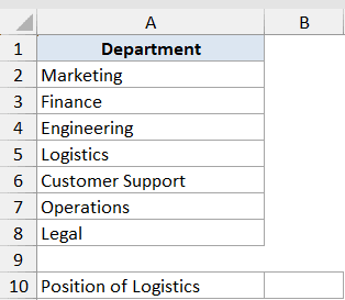
I want a single number that tells me where “Logistics” appears in the list.
Here is the formula:
=MATCH("Logistics", A2:A8, 0)
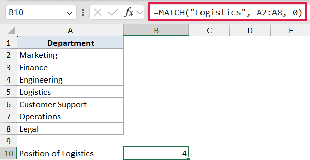
In the above formula, MATCH looks for “Logistics” in A2:A8 and returns its position. The third argument is 0, which forces an exact match. If “Logistics” is the fourth name in that range, the result is 4.
The position is relative to the lookup array, not to the worksheet, so MATCH does not care that the range starts at row 2.
Pro Tip: If you ever see MATCH return something odd (a position that’s clearly wrong), check that you passed 0 as the third argument. The default behavior assumes the data is sorted ascending, and it returns the position of the largest value less than or equal to your lookup value, not an exact match.
Example 2: Spill Positions for a Whole List
Here’s the dynamic-array version. Instead of looking up one value at a time, you can pass MATCH a whole column of lookup values and it returns the positions for all of them in one shot.
Below is a master list of product SKUs in column A (A2:A12), and a shorter list of SKUs to check in column D (D2:D6). I want to find where each SKU in D2:D6 sits inside the master list.
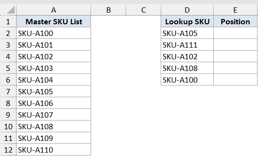
I want one formula that returns five position numbers, one for each SKU in D2:D6.
Here is the formula in E2:
=MATCH(D2:D6, A2:A12, 0)
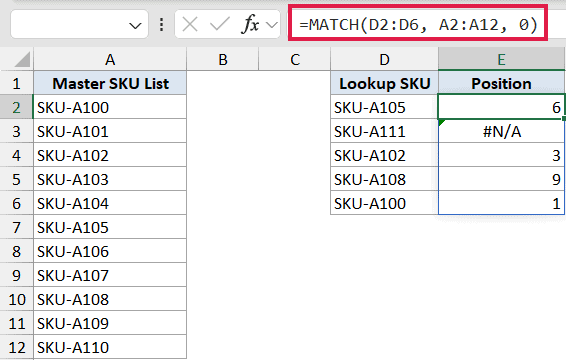
In the above formula, MATCH receives an array of five lookup values from D2:D6. In Excel 365, it returns an array of five positions that spills down from E2 to E6 automatically. No need to copy the formula down or use Ctrl+Shift+Enter.
In Excel 365, XMATCH does the same job and defaults to an exact match, so you can drop the third argument: =XMATCH(D2:D6, A2:A12). Same spilled output, one less argument to remember.
If any value in D2:D6 isn’t found in the master list, that row in the spill range shows #N/A. You can wrap the whole thing in IFERROR if you want a cleaner output: =IFERROR(MATCH(D2:D6, A2:A12, 0), "Not found").
Example 3: Two-Way Lookup with INDEX and MATCH
This is the classic combo that made MATCH famous. INDEX returns the value at a specific row and column position, and MATCH supplies those positions dynamically.
Below is a small grid of monthly sales by salesperson. Names sit in column A (A2:A6), months sit in row 1 (B1:G1), and the sales values fill the grid between them.
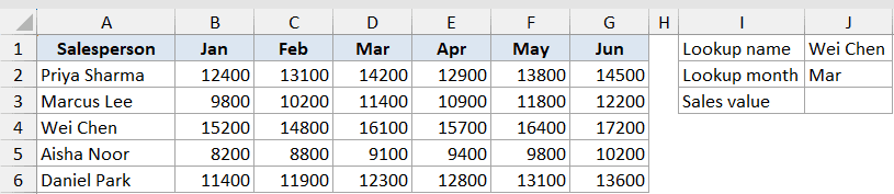
I want the sales value for a specific salesperson in a specific month, picked from two input cells (J1 holds the name and J2 holds the month).
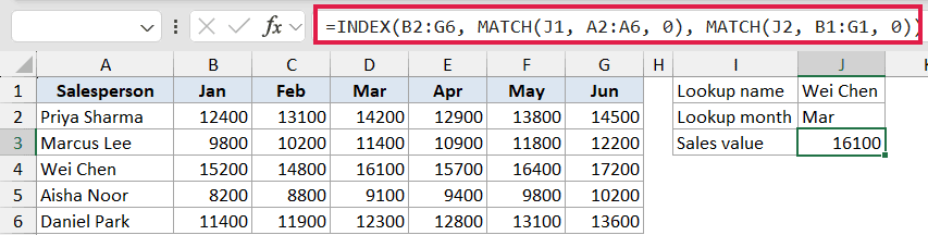
Here is the formula:
=INDEX(B2:G6, MATCH(J1, A2:A6, 0), MATCH(J2, B1:G1, 0))
How this formula works:
- The first MATCH looks for the salesperson name (in J1) inside A2:A6 and returns the row position. If the name is the third one in the list, MATCH returns 3.
- The second MATCH looks for the month (in J2) inside B1:G1 and returns the column position. If it’s the third column, MATCH returns 3.
- INDEX then pulls the value from B2:G6 at row 3, column 3.
In Excel 365, XLOOKUP handles the same job in a single nested call: =XLOOKUP(J1, A2:A6, XLOOKUP(J2, B1:G1, B2:G6)).
The INDEX/MATCH/MATCH version still works on every Excel version, though, so it’s worth knowing both.
If you’re curious how the two approaches compare side by side, XLOOKUP Vs INDEX MATCH in Excel walks through the trade-offs.
Example 4: Tier Lookup with Approximate Match
This is where the match_type = 1 argument earns its keep. You have a set of sorted thresholds and you want to drop a value into the right bracket.
It’s the same idea as finding the closest match below or equal to a target value.
Below is a shipping-rate table sorted ascending by order weight (in kg). Column A has weight thresholds (0, 5, 10, 20, 50) and column B has the rate for each tier. I want to find the right tier for an order weight in cell D2.
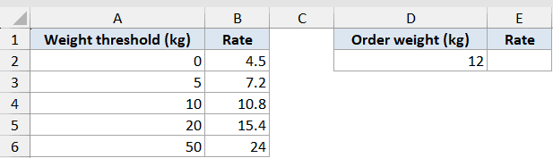
I want the position of the correct tier for the weight in G2 so I can pull the corresponding rate.
Here is the formula:
=INDEX(B2:B6, MATCH(D2, A2:A6, 1))
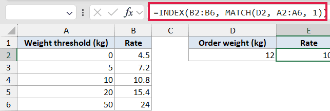
In the above formula, MATCH with match_type = 1 returns the position of the largest threshold in A2:A6 that is less than or equal to the weight in D2. If the weight is 12, MATCH returns 3 (the position of the 10 kg threshold), and INDEX then returns the rate for that tier from B2:B6.
This only works when the threshold column is sorted in ascending order. If it isn’t, MATCH will return wrong positions silently, which is one of the easiest bugs to introduce.
Example 5: Check Whether a Value Exists
You can flip MATCH into a simple check if value is in list by wrapping it in ISNUMBER. MATCH returns a number on success and #N/A on failure, so ISNUMBER turns that into a clean TRUE / FALSE.
Below is a list of email addresses from a recent newsletter signup in column A (A2:A15), and a shorter list of email addresses to check in column C (C2:C6). I want to flag whether each email in column C already exists in the signup list.
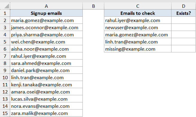
I want one formula in D2 that fills D2:D6 with TRUE or FALSE depending on whether each email is in the signup list.
Here is the formula:
=ISNUMBER(MATCH(C2:C6, A2:A15, 0))
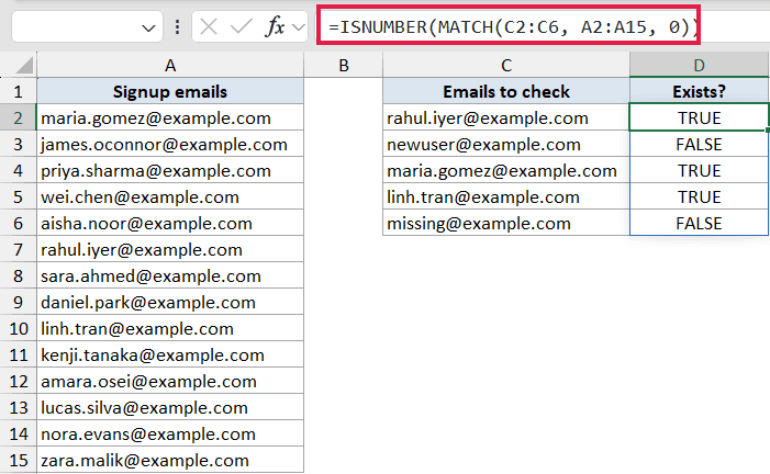
In the above formula, MATCH receives C2:C6 as an array of lookup values and returns an array of positions. For emails that exist in the signup list, the result is a number. For emails that don’t, it’s #N/A.
ISNUMBER converts both into TRUE or FALSE, and the whole thing spills down from D2 to D6.
If you want to count how many of the lookup emails exist, wrap it in SUM: =SUM(--ISNUMBER(MATCH(C2:C6, A2:A15, 0))). The double negative pushes TRUE/FALSE into 1/0 so SUM can total them.
This is a common existence check people reach for instead of COUNTIF when they need positions later.
Example 6: Wildcards for Partial-Text Match
When you only know part of the value you’re looking for, you can pass a wildcard into MATCH. The asterisk (*) matches any number of characters, and the question mark (?) matches a single character. Wildcards only work when match_type is 0.
Below is a list of customer support ticket subjects in column A (A2:A10). I want to find the position of the first ticket that mentions “refund” anywhere in the subject.
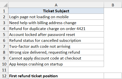
I want the position of the first ticket subject that contains the word “refund”.
Here is the formula:
=MATCH("*refund*", A2:A10, 0)
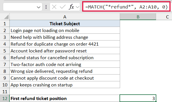
In the above formula, the asterisks tell MATCH to match any text before or after “refund”. The first subject that contains the word gets returned as a position, and MATCH is case-insensitive so “Refund” and “REFUND” hit the same way.
Wrap this in INDEX if you want the actual subject line: =INDEX(A2:A10, MATCH("*refund*", A2:A10, 0)).
Pro Tip: If you actually need to search for a literal asterisk or question mark, prefix it with a tilde: ~* or ~?. Otherwise Excel treats them as wildcards.
Tips & Common Mistakes
- Always pass 0 as the third argument unless you specifically need an approximate match. The default behavior is
match_type = 1, which assumes the data is sorted ascending and returns the largest value less than or equal to the lookup value. People skip the third argument, get a wrong-looking result on unsorted data, and lose half an hour finding the bug. - #N/A means the value wasn’t found. The most common causes are a typo, an extra space (run TRIM on the data), or a mismatch between numbers stored as text and numbers stored as numbers. Wrap MATCH in IFERROR to handle missing values cleanly.
- MATCH is case-insensitive. “logistics” and “Logistics” return the same position. If you need a case-sensitive match, you need a different formula (EXACT inside an array MATCH, for example).
- Modern alternatives: On Excel 365 and 2021, XMATCH is the upgraded version. It defaults to exact match, supports reverse-search (find the last match instead of the first), and has a binary-search mode for large sorted lists. The INDEX/MATCH/MATCH two-way lookup pattern is cleanly handled by nested XLOOKUP calls. The classic MATCH formulas above still work everywhere, so they’re worth knowing for older Excel versions and inherited workbooks.
- Lookup_array must be one row or one column. MATCH does not work on a two-dimensional range. If you pass it B2:G6, you’ll get a #N/A or unexpected results. Pair two MATCH calls (one for rows, one for columns) with INDEX for the grid case.
That covers the main ways MATCH gets used in real spreadsheets: position lookups, INDEX/MATCH two-way pulls, tier matching, existence checks, and wildcard searches.
MATCH is a small function but it shows up everywhere once you start building lookups that need to be flexible about direction or array input. Pair it with INDEX or XLOOKUP and you’ll cover almost every lookup case Excel throws at you.
Related Excel Functions / Articles:
- LOOKUP Function in Excel
- SEARCH Function in Excel
- CHOOSE Function in Excel
- IFNA Function in Excel
- ISNA Function in Excel
- OFFSET Function in Excel
- Using VLOOKUP Approximate Match in Excel (Examples)
- How to Compare Two Cells in Excel? (Exact/Partial Match)
- INDEX Function in Excel
- VLOOKUP Function in Excel
- INDEX MATCH with Multiple Criteria in Excel