
The EXACT function in Excel returns TRUE when two text strings match exactly, including letter case, and FALSE otherwise.
It can identify differences in codes or names that an ordinary equality comparison overlooks. Differences in cell formatting do not affect the comparison.
In this article, I’ll show you how to compare text with case sensitivity, count exact matches, and perform a case-sensitive lookup.
EXACT Function Syntax in Excel
The EXACT function takes two text strings and returns a logical value (TRUE or FALSE) based on whether they match exactly.
=EXACT(text1, text2)
- text1: The first text string you want to compare.
- text2: The second text string you want to compare.
EXACT is case-sensitive and treats whitespace as part of the string. It ignores most cell formatting (currency, number, percentage), but compares the underlying values.
When to Use EXACT Function
Use the EXACT function when:
- You need a case-sensitive way to compare two cells or two columns of text.
- You’re verifying passwords, product codes, SKUs, or user IDs where case matters.
- You want to flag rows where the visible text looks the same but differs by case or hidden whitespace.
- You’re building a case-sensitive lookup or count, since VLOOKUP, XLOOKUP, and COUNTIF are all case-insensitive by default.
- You’re validating that entries follow a format rule, like all-uppercase or proper-case.
Example 1: Compare Two Columns Side by Side
Let’s start with the most common use case for EXACT, comparing two columns of text side by side.
Below is the dataset. Column A is a list of customer names as recorded by a vendor, and column B is the same list as stored internally. We want to check whether the two lists match exactly, row by row.
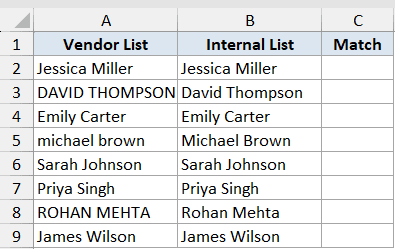
I want to flag every row where the vendor’s name differs from the internal name in any way, including capitalization.
Here is the formula:
=EXACT(A2:A9, B2:B9)
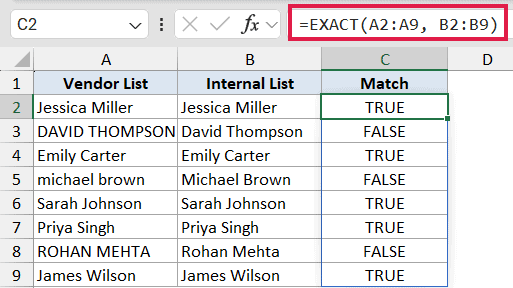
This is a single formula entered in C2 that spills the TRUE/FALSE results across cells C2 through C9. For each row, EXACT compares the vendor name to the internal name character by character, including case.
Rows like DAVID THOMPSON against David Thompson return FALSE, even though they’re technically the same person.
Pro Tip: If you’re on Excel 2019 or earlier, the spilling version won’t work. Type =EXACT(A2, B2) into C2 and drag it down to C9 to get the same result.
Example 2: EXACT vs the = Operator
Here’s a good way to see what EXACT does that the equals operator (=) doesn’t.
Below is the dataset. Column A and column B both contain short text values. Some pairs differ in case, some in spacing, and some are genuinely identical.
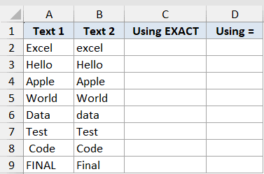
I want to compare each pair using both = and EXACT, side by side, to see where the two approaches give different answers.
Here are the formulas:
=EXACT(A2:A9, B2:B9)
=A2:A9=B2:B9
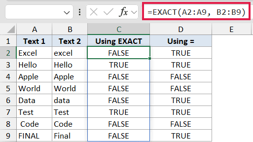
The first formula (in column C) uses EXACT. It returns TRUE only when both strings match character for character, including case and whitespace.
The second formula (in column D) uses the equals operator. It returns TRUE whenever the two strings match in a case-insensitive way, but FALSE when there’s any whitespace difference.
Look at row 2: Excel vs excel. EXACT returns FALSE (because the case differs), but the = operator returns TRUE (it ignores case). That’s the difference in one row.
Scan down the two columns and you can see exactly which mismatches each method catches and which ones it misses.
Pro Tip: Both = and EXACT flag a leading or trailing space as a mismatch. If you want to ignore whitespace differences, wrap both sides in TRIM, like =EXACT(TRIM(A2), TRIM(B2)).
Example 3: Password Match with IF + EXACT
Now let’s wrap EXACT in IF to turn a TRUE/FALSE result into something more useful, like an access-control verdict.
Below is the dataset. Column A holds passwords entered by users, and column B holds the matching stored password for each user. Some entries match exactly; others have casing typos.
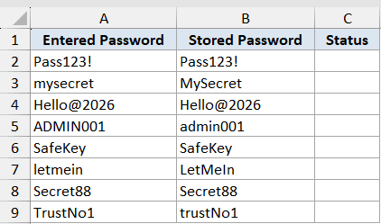
I want to spill a Granted or Denied status down column C based on whether the entered password matches the stored password exactly.
Here is the formula:
=IF(EXACT(A2:A9, B2:B9), "Granted", "Denied")
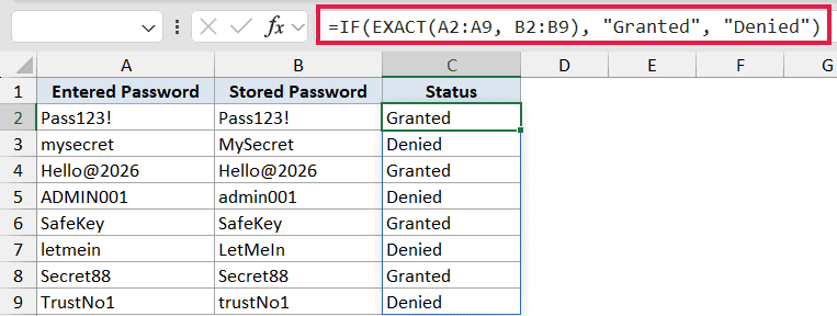
EXACT returns an array of TRUE/FALSE values, one per row. IF wraps that array and returns Granted for each TRUE and Denied for each FALSE. Because the formula is entered in C2 and feeds in ranges, the result spills down to C9 automatically.
Notice that mysecret against MySecret returns Denied. A regular = comparison would have let that one through because = ignores case.
Pro Tip: Real password verification should never store plaintext passwords. This example is just to illustrate how IF + EXACT works for case-sensitive matching, which is useful for product codes, SKUs, license keys, and similar identifiers.
Example 4: Count Case-Sensitive Matches
COUNTIF can count how many times a value appears in a range, but it’s case-insensitive. To count case-sensitive matches, EXACT plus SUMPRODUCT is the standard trick.
Below is the dataset. Column A holds a list of project codes, some uppercase, some lowercase, some mixed. We want to count how many cells exactly match the target code AB1 (not ab1, not Ab1).
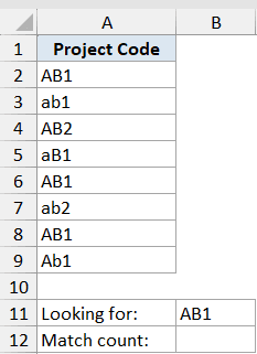
The target code is sitting in B11, and I want the count to land in B12.
Here is the formula:
=SUMPRODUCT(--EXACT(A2:A9, B11))
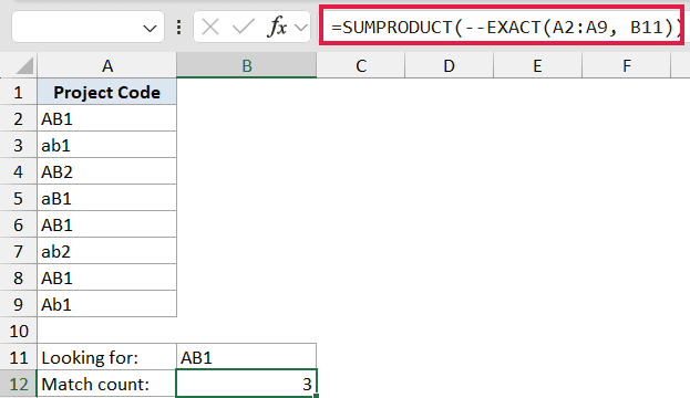
EXACT compares each project code in A2:A9 to the target in B11 and returns an array of TRUE/FALSE values. The double negative (--) converts TRUE to 1 and FALSE to 0. SUMPRODUCT then sums the 1s, which gives you the count of exact matches.
The result is 3, because only three cells contain the exact string AB1. A regular =COUNTIF(A2:A9, B11) would return 6 here, since COUNTIF treats AB1, ab1, Ab1, and aB1 as the same value.
In Excel 365, you can also use =SUM(–EXACT(A2:A9, B11)) since SUM accepts array expressions now. SUMPRODUCT is the safer pick if anyone might open this workbook in Excel 2019 or earlier.
Example 5: Case-Sensitive Lookup
VLOOKUP and XLOOKUP are both case-insensitive. If you need a case-sensitive lookup, INDEX, MATCH, and EXACT work together to do the job.
Below is the dataset. Column A holds user IDs, and column B holds the matching email address for each user. The IDs aReynolds and AReynolds are two different users.
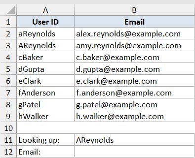
The lookup target is in B11 (AReynolds), and I want the email for that exact user, not for aReynolds.
Here is the formula:
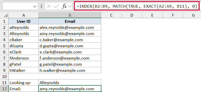
=INDEX(B2:B9, MATCH(TRUE, EXACT(A2:A9, B11), 0))
How this formula works:
EXACT(A2:A9, B11)returns an array of TRUE/FALSE values, one per user ID compared to the target. The only TRUE is at position 2, where AReynolds lives.MATCH(TRUE, <array>, 0)finds the position of the first TRUE in that array, which is 2.INDEX(B2:B9, 2)returns the value at row 2 of the email column, which is amy.reynolds@example.com.
If you’d used VLOOKUP or XLOOKUP here, you’d have gotten alex.reynolds@example.com (the first match ignoring case), which is the wrong user.
In Excel 365, you can also write this as =FILTER(B2:B9, EXACT(A2:A9, B11)), which returns the same email in one cleaner step. The INDEX + MATCH version still works in older Excel, so it’s worth knowing both.
Example 6: Validate Uppercase Entry
EXACT pairs well with UPPER, LOWER, and PROPER when you need to check whether a column of entries follows a case convention.
Below is the dataset. Column A holds product codes that should all be uppercase, but a few entries slipped through with lowercase or mixed-case letters.
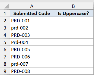
I want column B to show TRUE for codes that are fully uppercase and FALSE for codes that aren’t.
Here is the formula:
=EXACT(A2:A9, UPPER(A2:A9))
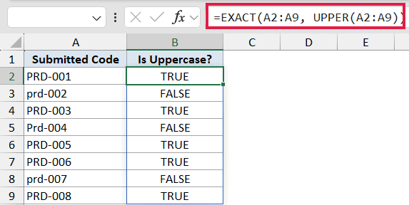
UPPER(A2:A9) returns an array of uppercase versions of each code. EXACT compares the original code in column A to its uppercase version. If the two match, the code is already uppercase (TRUE); if they don’t, the code has at least one lowercase letter (FALSE).
This is a quick way to audit a column of codes, SKUs, or identifiers for casing mistakes before importing the data into another system.
Tips & Common Mistakes
- EXACT only takes two arguments. If you need to compare more than two strings, nest EXACT inside an AND function, like =AND(EXACT(A2,B2), EXACT(B2,C2)).
- EXACT is case-sensitive but also whitespace-sensitive. A trailing space, leading space, or extra space in the middle counts as a mismatch. If you don’t want spaces to break the match, wrap both arguments in TRIM.
- EXACT ignores most cell formatting (currency, percentage, number formats), but treats dates and times as their underlying serial numbers. Two cells showing the same date can match even if one is formatted as a long date and the other as a short date.
- The equals operator (=) is case-insensitive, so use EXACT whenever case matters. This is especially important for passwords, SKUs, license keys, and any identifier where AB1 and ab1 represent different things.
- In Excel 365, EXACT spills naturally when fed two ranges of the same shape. In Excel 2019 and earlier, you’ll need to either copy the formula down each row or enter it with Ctrl+Shift+Enter as an array formula.
- COUNTIF, SUMIF, VLOOKUP, and XLOOKUP are all case-insensitive. For case-sensitive counts use SUMPRODUCT + EXACT, and for case-sensitive lookups use INDEX + MATCH + EXACT, or FILTER + EXACT in 365.
The EXACT function is small but handy whenever case sensitivity matters in your text comparisons. You can drop it in directly for two cells, or spill it across two columns in Excel 365.
Pair it with SUMPRODUCT, INDEX/MATCH, IF, and UPPER for case-sensitive counts, lookups, conditional outputs, and format checks.
Once you start using EXACT, you’ll notice all the places where Excel’s default case-insensitive comparison was quietly letting differences slip through.
Related Excel Functions / Articles:
- How to Compare Two Columns in Excel (using VLOOKUP & IF)
- XLOOKUP Vs INDEX MATCH in Excel
- How to Change Uppercase to Lowercase in Excel
- Bulk Find and Replace in Excel
- Count How Many Times a Word Appears in Excel (Easy Formulas)
- Wildcard Characters in Excel
- SEARCH vs FIND Function in Excel
- Microsoft Excel Terminology (Glossary)
