
If you’re running a hypothesis test, sooner or later you need a critical value to decide whether your result is actually significant. The tricky part is that Excel has no single “critical value” button.
The right function depends on which distribution your test uses. Once you know that, it’s a one-line formula. Below I’ll show you four of them, covering the Z, t, chi-square, and F tests.
Method #1: Using the NORM.S.INV Function
NORM.S.INV gives you the critical value from the standard normal (Z) distribution. You’d reach for this when your sample is large or the population standard deviation is already known, which is when a Z-test applies.
To keep a running example, I have exam scores for 12 students split across three class sections. I’ll come back to these same three sections in every method.
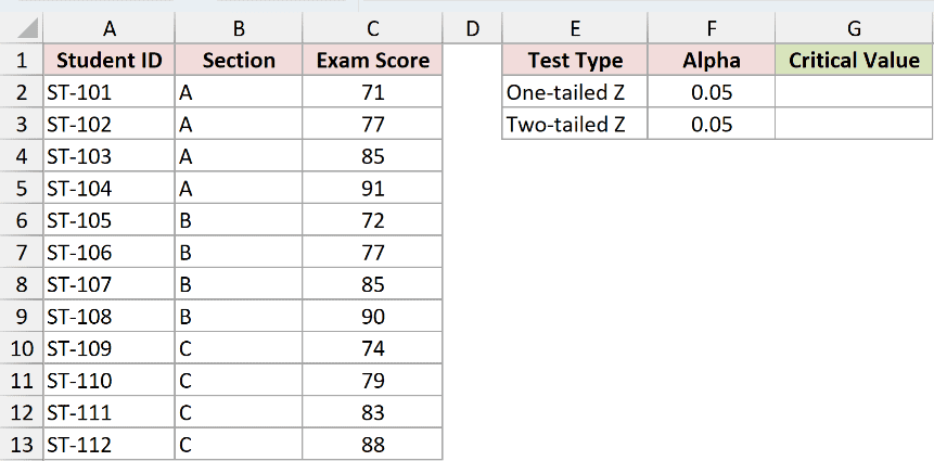
I’ll note my significance level (alpha), 0.05, in a cell so it stays visible next to the result. A Z critical value only needs alpha, since the standard normal distribution has no degrees of freedom.
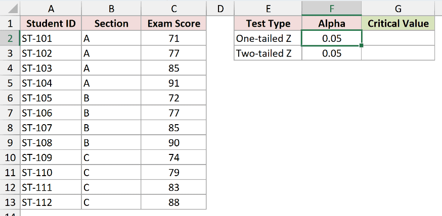
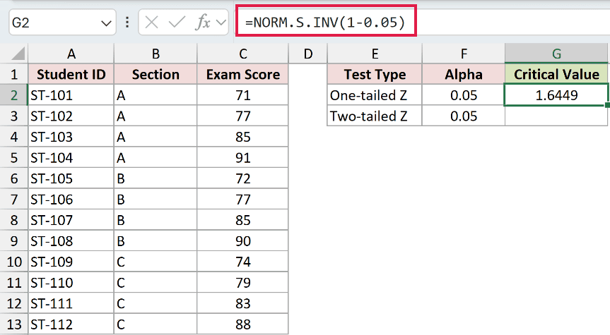
For a one-tailed test at 5%, here is the formula:
=NORM.S.INV(1-0.05)
This returns 1.6449. That’s the upper-tail critical value. If your test is in the lower tail instead, the matching value is its negative, -1.6449.
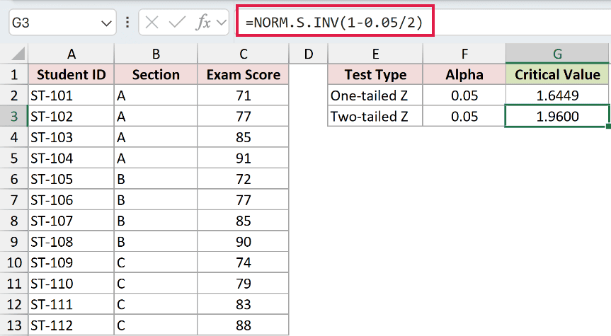
For a two-tailed test, you split alpha across both tails, so each tail holds 0.025. That means you feed in 1-0.05/2:
=NORM.S.INV(1-0.05/2)
This returns 1.96, the familiar two-tailed Z value at 95% confidence.
How does this formula work?
NORM.S.INV is the inverse of the standard normal curve. You hand it a cumulative probability and it returns the z-score that has that much area to its left.
For a one-tailed 5% test you want the z with 95% of the area below it, so you pass 1-0.05. For two tails you want 97.5% below, so you pass 1-0.05/2.
Note: Use the Z critical value only when your sample is large or the population standard deviation is known. For my 12-student sample with an unknown population spread, the t critical value in Method #2 is the correct choice.
Method #2: Using the T.INV.2T Function
This is the one you’ll use most often, so it’s the method I’d recommend by default. T.INV.2T gives the two-tailed critical value from the t-distribution, which is what you need for a two-tailed t-test when the population standard deviation is unknown.
Say I want to check whether my class average is significantly different from the school’s pass benchmark of 75. That’s a two-tailed question, and with a small sample the t-distribution is the honest choice.
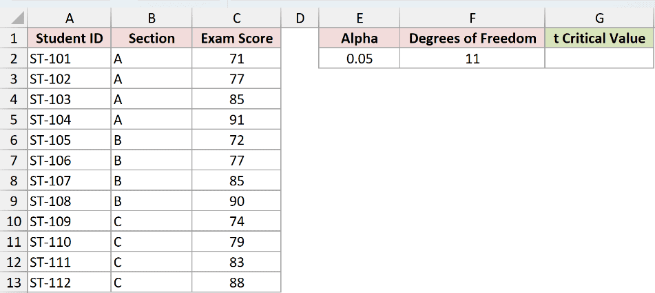
A t critical value needs two inputs: alpha and the degrees of freedom. For a one-sample test the degrees of freedom are the sample size minus one, so 12 – 1 = 11.
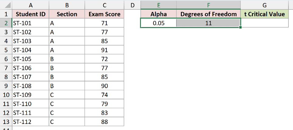
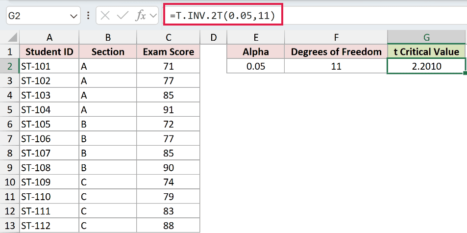
Here is the formula:
=T.INV.2T(0.05,11)
This returns 2.2010. So the two critical values are +2.2010 and -2.2010, and any test statistic beyond that range is significant.
How does this formula work?
My 12 scores have a mean of 81 and a sample standard deviation of about 6.95, which you get from STDEV.S, not STDEV.P.
The one-sample t statistic is (81 – 75) divided by (6.95 / the square root of 12), which works out to roughly 2.99.
Since the absolute value of 2.99 is greater than 2.2010, the result lands in the rejection region. The sample provides statistically significant evidence that the class average differs from 75 at the 5% level.
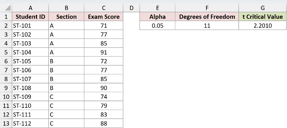
Note: T.INV.2T already splits alpha across both tails, so pass the full 0.05, not 0.05/2. For a one-tailed t critical value use =T.INV(1-0.05,11) instead, which returns 1.7959. A one-sample t-test also assumes independent observations and a roughly normal population, especially with only 12 scores.
Method #3: Using the CHISQ.INV.RT Function
If you’d rather test categories than averages, this is the function for you. CHISQ.INV.RT returns the right-tailed critical value from the chi-square distribution, used for goodness-of-fit and independence tests.
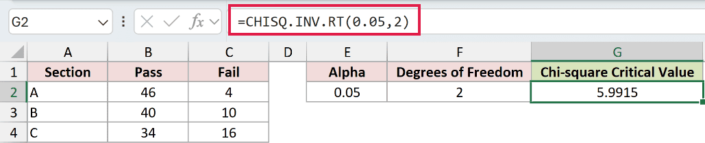
This time, instead of the 12-score sample, I’ve pulled the full semester results for the same three sections. Each section had 50 students take the exam, and I’ve counted how many passed and how many failed in each. The question is whether passing is independent of the section a student is in. That’s a chi-square test of independence.

For a test of independence, the degrees of freedom are (rows – 1) multiplied by (columns – 1). With 3 sections and 2 outcomes that’s (3 – 1) times (2 – 1), which equals 2.

Here is the formula:
=CHISQ.INV.RT(0.05,2)
This returns 5.9915. If your calculated chi-square statistic climbs above 5.9915, you reject the idea that the two categories are independent.
How does this formula work?
The chi-square distribution only has a meaningful right tail here, so CHISQ.INV.RT takes the tail probability directly. Pass it alpha and the degrees of freedom, and it returns the cutoff with 5% of the area to its right.
To use that cutoff, you need the chi-square statistic from the table. With 120 passes spread over three equal sections of 50, the expected counts are 40 passes and 10 fails per section. Take each cell’s gap between observed and expected, square it, and divide by the expected count. Across the six cells that gives 0.9, 3.6, 0, 0, 0.9, and 3.6, which adds up to 9.00.
Since 9.00 is greater than 5.9915, the result lands in the rejection region. Passing is not independent of section here, and you can see why. Section A fails only 4 students out of 50 while Section C fails 16.
Note: A chi-square test wants every expected count to be at least 5. This table clears that bar comfortably, since the smallest expected count is 10. Always check this before trusting the result on a smaller dataset.
Method #4: Using the F.INV.RT Function
When you’re comparing more than two groups at once, you’re usually running ANOVA, and that needs an F critical value. F.INV.RT returns the right-tailed cutoff from the F distribution.
Here I’d use it to compare the average scores across all three sections in one test, rather than checking two sections at a time.
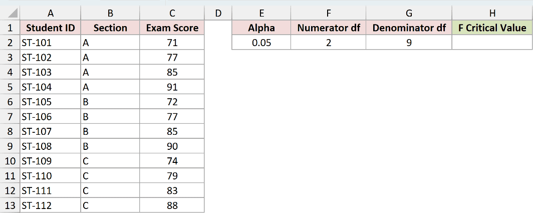
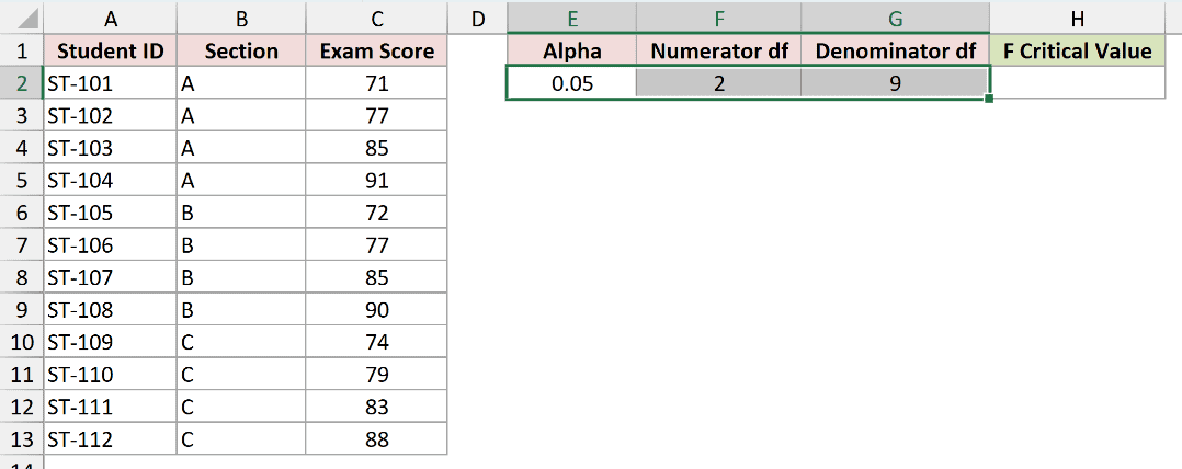
The F distribution takes two separate degrees of freedom. For one-way ANOVA the first is the number of groups minus one (3 – 1 = 2), and the second is the total sample size minus the number of groups (12 – 3 = 9).
Here is the formula:
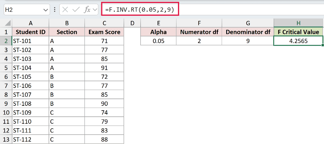
=F.INV.RT(0.05,2,9)
This returns 4.2565. If the F statistic from your ANOVA output is larger than 4.2565, at least one section mean differs from the others. If it’s smaller, you fail to reject the null hypothesis, but that does not prove the section means are the same.
How does this formula work?
F.INV.RT is right-tailed like its chi-square cousin, so the first argument is the tail probability. The two degrees-of-freedom arguments must go in the right order: the numerator (between-groups) value first, then the denominator (within-groups) value.
Note: Swapping the two degrees-of-freedom arguments changes the answer, since the F distribution isn’t symmetric. Numerator degrees of freedom always go before the denominator ones.
Additional Notes About Finding Critical Values in Excel
- Match the function to your test’s distribution. A Z-test uses
NORM.S.INV, a t-test usesT.INV.2T, a chi-square test usesCHISQ.INV.RT, and an F-test or ANOVA usesF.INV.RT. Pick the wrong one and the cutoff is meaningless. - Know which tail the function assumes. The
.RTfunctions are right-tailed and take the tail probability directly.NORM.S.INVandT.INVare left-tailed, so you feed them1-alpha, not alpha. - In your own sheets, consider keeping alpha and degrees of freedom in cells and pointing the formulas at them, like =T.INV.2T($F$2,$G$2). A single edit then updates every critical value, which is handy when you want to compare 0.05 against 0.01. In this tutorial I’ve typed the values directly so each formula stands on its own.
- The older function names still work. Excel keeps
NORMSINV,TINV, andCHIINVfor backward compatibility, but the newer dotted versions are clearer about which tail they use.
Frequently Asked Questions
What’s the difference between a critical value and a p-value?
A critical value is a fixed cutoff you set before the test from your alpha and distribution. A p-value comes out of your data.
You compare your test statistic to the critical value, or compare the p-value to alpha, and both roads reach the same decision.
Do I need the Data Analysis ToolPak to find critical values in Excel?
No. Every function shown here is built into Excel, so you can type them straight into a cell. The ToolPak helps you run the full test, but the critical value itself is just a formula.
How do I know if I need a one-tailed or two-tailed critical value?
Use one-tailed when your question has a direction (“is the average higher than 75?”). Use two-tailed when you only care whether there’s any difference in either direction (“is the average different from 75?”). Two-tailed is the safer default when you’re unsure.
Conclusion
Finding a critical value in Excel comes down to picking the function that matches your test’s distribution, then feeding it your alpha and degrees of freedom.
For everyday work the two-tailed t critical value from T.INV.2T is the one you’ll type most, so that’s where I’d start. Keep NORM.S.INV, CHISQ.INV.RT, and F.INV.RT in your back pocket for Z, chi-square, and ANOVA tests.
Other Excel articles you may also like:
