
If you want to multiply two sets of related values and return several totals at once, the MMULT function is built for the job.
In this article, I’ll show you how to use MMULT for revenue, costs, totals, running totals, weighted scores, and payroll.
MMULT is a dynamic array function, and it spills its results across the cells below or beside the formula.
MMULT Function Syntax in Excel
The MMULT function multiplies two arrays and returns their matrix product.
=MMULT(array1,array2)
- array1 (required) is the first array of numbers.
- array2 (required) is the second array of numbers.
- The number of columns in array1 must equal the number of rows in array2.
- The result has the same number of rows as array1 and the same number of columns as array2.
When to Use MMULT Function
- Calculate revenue or cost totals from quantities and unit values.
- Return several related calculations from two tables with one formula.
- Add rows or columns by multiplying a data array by a vector of ones.
- Build running totals with a lower-triangular matrix.
- Calculate weighted scores for several records at once.
- Solve a system of linear equations by pairing MMULT with MINVERSE.
Example 1: Calculate Revenue per Store
Let’s start with a practical matrix-times-vector calculation.
Below is the dataset. Columns B to D contain unit sales by store, and H2:H4 contains the corresponding unit prices.
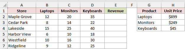
We want to calculate total revenue for every store with one formula in E2.
Here is the formula:
=MMULT(B2:D7,H2:H4)
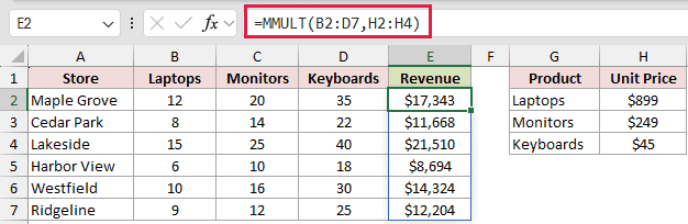
The sales range is a 6 by 3 array, while the price range is a 3 by 1 array.
MMULT pairs each store’s three quantities with the three prices. The resulting 6 by 1 array spills from E2 through E7.
The revenues are $17,343, $11,668, $21,510, $8,694, $14,324, and $12,204.
Pro Tip: Keep E2:E7 empty before entering the formula. Any existing value in that output range causes a #SPILL! error.
Example 2: Multiply Two Matrices
Now let’s return two calculations for each cafe from the same formula.
Below is the dataset. B2:D4 contains order quantities, while G2:H4 contains each product’s unit cost and unit price.

We want to calculate total cost and total revenue for all three cafes.
Here is the formula:
=MMULT(B2:D4,G2:H4)

This time, a 3 by 3 order array is multiplied by a 3 by 2 cost-and-price array.
The result is a 3 by 2 grid. Its rows match the cafes, and its columns return total cost and total revenue.
Downtown returns $290.00 and $735.00. Riverside returns $252.50 and $645.00, while Uptown returns $336.00 and $847.50.
This output shape is worth remembering. MMULT returns the rows of the first array by the columns of the second array.
Example 3: Calculate Row and Column Totals
Here’s a less obvious way to total quarterly sales without filling SUM formulas across the sheet.
Below is the dataset. B2:E7 contains quarterly sales for six representatives, with space for row and column totals.
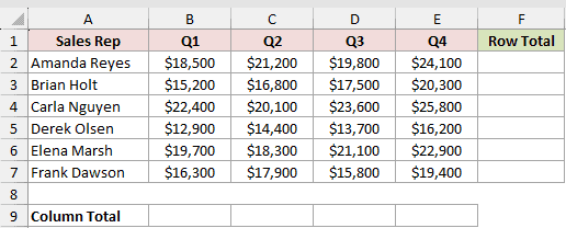
We first want to add the four quarterly values on every row.
Here is the row-total formula:
=MMULT(B2:E7,SEQUENCE(4,1,1,0))
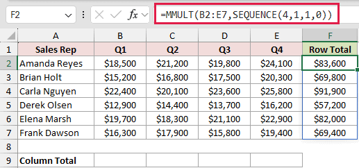
SEQUENCE(4,1,1,0) creates a 4 by 1 array containing four ones. MMULT multiplies every sales row by that vector and spills six totals.
The row totals are $83,600, $69,800, $91,900, $57,200, $82,000, and $69,400.
We also want to add the six values in each quarterly column.
Here is the column-total formula:
=MMULT(SEQUENCE(1,6,1,0),B2:E7)
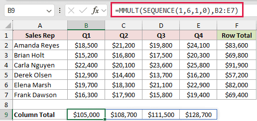
The first SEQUENCE now creates a 1 by 6 row of ones. MMULT returns four totals across B9:E9.
The quarterly totals are $105,000 for Q1, $108,700 for Q2, $111,500 for Q3, and $128,700 for Q4.
In Excel 365, =BYROW(B2:E7,LAMBDA(r,SUM(r))) and =BYCOL(B2:E7,LAMBDA(c,SUM(c))) are more direct for this job.
The MMULT versions also fit naturally inside larger matrix calculations.
Example 4: Create a Running Total
Let’s use a calculated matrix to turn weekly deposits into a running total.
Below is the dataset. B2:B9 contains eight weekly deposits, while columns C and D compare MMULT with SCAN.
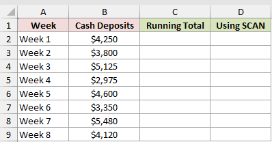
We want each row in column C to include the current deposit and every deposit above it.
Here is the MMULT formula:
=MMULT(--(ROW(B2:B9)>=TRANSPOSE(ROW(B2:B9))),B2:B9)
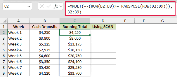
ROW(B2:B9)>=TRANSPOSE(ROW(B2:B9)) creates an 8 by 8 lower-triangular array of TRUE and FALSE values.
The double unary converts those values to ones and zeros. Each matrix row then includes one more deposit than the row above it.
The running total starts at $4,250, reaches $20,750 in Week 5, and ends at $33,700 in Week 8.
In Excel 365, here is the modern SCAN formula for comparison:
=SCAN(0,B2:B9,LAMBDA(a,v,a+v))
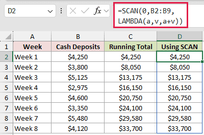
SCAN carries the previous total into each new calculation, so it produces the same eight results with a shorter formula.
Use SCAN when you only need a running total.
Example 5: Calculate Weighted Candidate Scores
Now let’s calculate interview scores using different weights for three criteria.
Below is the dataset. B2:D7 contains candidate scores, and I2:I4 contains weights of 50%, 30%, and 20%.

We want one formula to return the weighted score for all six candidates.
Here is the MMULT formula:
=MMULT(B2:D7,I2:I4)
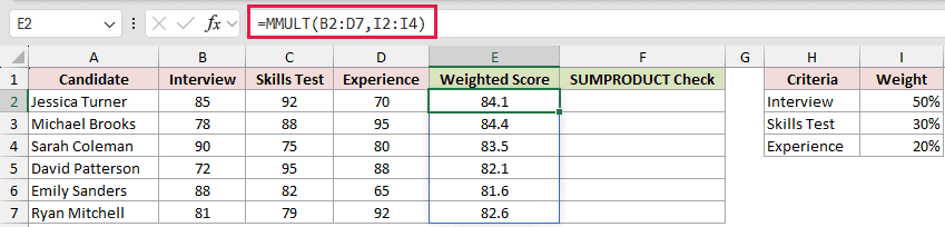
MMULT multiplies every interview, skills test, and experience score by its corresponding weight, then adds those products for each candidate.
The weighted scores are 84.1, 84.4, 83.5, 82.1, 81.6, and 82.6. Michael Brooks has the highest score at 84.4.
And here is a SUMPRODUCT check for the first candidate:
=SUMPRODUCT(B2:D2,TRANSPOSE($I$2:$I$4))
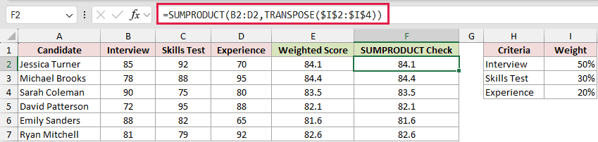
Copy this formula down through F7. The absolute references keep the weight range fixed while the candidate score range moves to each row.
SUMPRODUCT is often clearer for one weighted score. MMULT is more convenient when you want the full column returned by one spilling formula.
Example 6: Fix the #VALUE! Error
Finally, let’s fix the dimension mismatch that causes many MMULT errors.
Below is the dataset. B2:D5 contains task hours, and H2:J2 contains the three hourly rates as a horizontal row.

We first want to see why multiplying the hours by the rate row fails.
Here is the formula that returns #VALUE! in H4:
=MMULT(B2:D5,H2:J2)

The hours array has three columns, but the rate array has only one row. Those inner dimensions must match, so MMULT returns #VALUE!.
We want to turn the 1 by 3 rate row into a 3 by 1 column before multiplying.
Here is the corrected formula:
=MMULT(B2:D5,TRANSPOSE(H2:J2))

TRANSPOSE changes the orientation without moving the source values. MMULT can then multiply the 4 by 3 hours array by the 3 by 1 rates array.
The four total pay amounts spill into E2:E5 as $2,875, $3,020, $2,860, and $2,680.
Pro Tip: When MMULT returns #VALUE!, compare the number of columns in array1 with the number of rows in array2 first.
Tips & Common Mistakes
- MMULT requires numeric arrays. Text, blank cells, or other nonnumeric values inside either array return #VALUE!.
- Check the inner dimensions before entering the formula. The columns in the first array must equal the rows in the second array.
- Keep the complete spill range empty in Excel 365. A blocked output cell causes #SPILL!.
- In Excel 2019 and earlier, select the complete output range first and confirm MMULT with Ctrl+Shift+Enter.
- Use ordinary multiplication when you need element-by-element products. MMULT calculates a matrix product, which follows different dimension and calculation rules.
- SUMPRODUCT is usually easier for one row, while MMULT is useful when one formula must return several related results.
We covered revenue by store, cost and revenue together, row and column totals, running totals, weighted scores, and a TRANSPOSE fix for mismatched dimensions.
Check the array shapes first, and the formula becomes much easier to build and troubleshoot.
Related Excel Functions / Articles:
