
If you want to summarize a list by both rows and columns, PIVOTBY builds the entire grid with one formula.
In this article, I’ll show you how to total, average, sort, filter, and calculate percentages with PIVOTBY.
PIVOTBY is a dynamic array function. It spills its whole summary grid from one cell.
PIVOTBY Function Syntax in Excel
PIVOTBY groups values by row and column fields, then applies an aggregation function to each intersection.
=PIVOTBY(row_fields, col_fields, values, function, [field_headers], [row_total_depth], [row_sort_order], [col_total_depth], [col_sort_order], [filter_array], [relative_to])
- row_fields (required) contains the categories you want to group into rows. You can supply one column or several adjacent columns.
- col_fields (required) contains the categories you want to group into columns. You can supply one column or several adjacent columns.
- values (required) contains the numbers or other values you want to summarize.
- function (required) is the calculation to apply, such as SUM, AVERAGE, or PERCENTOF.
- field_headers (optional) controls headers. Use 0 for none, 1 to hide existing headers, 2 to generate headers, or 3 to show existing headers. Omit it for automatic handling.
- row_total_depth (optional) controls the horizontal total rows. Use 0 for none, 1 for a grand total, or 2 for subtotals and a grand total.
- row_sort_order (optional) sets the row sorting field. Use a negative number for descending order.
- col_total_depth (optional) controls the vertical total columns. It uses the same depth values as row_total_depth.
- col_sort_order (optional) sets the column sorting field. Use a negative number for descending order.
- filter_array (optional) is a Boolean array that decides which source rows are included.
- relative_to (optional) sets PERCENTOF’s base: 0 for column totals (default), 1 for row totals, 2 for grand totals, 3 for parent column totals, or 4 for parent row totals.
PIVOTBY is available in Excel for Microsoft 365 on Windows, Mac, and the web. It is not available in Excel 2021 or Excel 2024 perpetual versions.
When to Use PIVOTBY Function
- Create a two-way summary without building helper formulas across a grid.
- Recalculate a summary automatically when source values change.
- Switch between totals, averages, percentages, and other supported calculations.
- Control total rows, total columns, sorting, and source-row filtering inside one formula.
- Build a formula-based alternative when you do not need the interactive controls of a PivotTable.
Example 1: Create a Two-Way Sales Summary
Let’s start with the four required arguments.
Below is the dataset. Column A lists crew leads, column B lists services, and column C contains invoice amounts for 12 landscaping jobs.
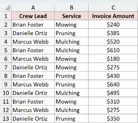
We want to total invoice amounts for every crew lead and service combination.
Here is the formula:
=PIVOTBY(A2:A13,B2:B13,C2:C13,SUM)
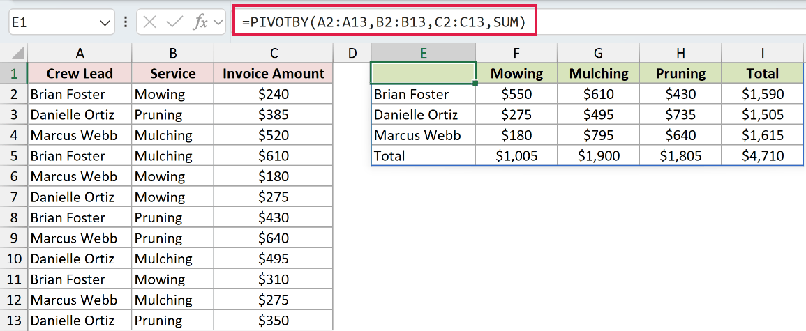
The first range creates the row labels, the second creates the column labels, and the third supplies the values. SUM adds each matching group.
The formula in E1 spills through I5. Brian Foster’s total is $1,590, while the grand total in I5 is $4,710.
The blank cell at E1 is correct. It is the corner where the row labels and column labels meet in the spilled grid.
Pro Tip: Clear the entire destination area before entering the formula. Any occupied cell inside E1:I5 blocks the grid and causes a #SPILL! error.
Example 2: Calculate Averages by Two Fields
Now let’s change the calculation without rebuilding the summary.
Below is the dataset. Column A lists real estate agents, column B shows property types, and column C contains days on market.
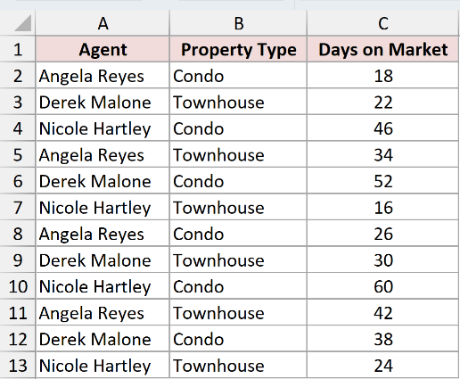
We want the average days on market for each agent and property type.
Here is the formula:
=PIVOTBY(A2:A13,B2:B13,C2:C13,AVERAGE)
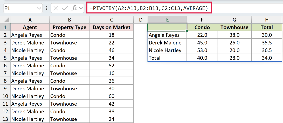
Only the fourth argument changes from SUM to AVERAGE. PIVOTBY keeps the same two-way layout and averages the matching days instead.
Angela Reyes averages 22.0 days for condos and 38.0 for townhouses. Her overall average is 30.0 days.
The Total row shows 40.0 days for condos, 28.0 for townhouses, and 34.0 overall.
Example 3: Remove Total Rows and Columns
Here’s a cleaner output when the summary will feed a chart.
Below is the dataset. Columns A and B identify each building and quarter, while column C contains utility costs.
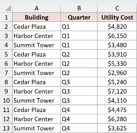
We want a building-by-quarter grid without a Total row or Total column.
Here is the formula:
=PIVOTBY(A2:A13,B2:B13,C2:C13,SUM,,0,,0)
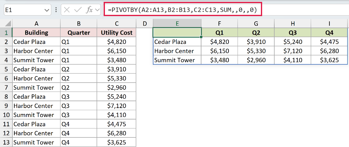
The first 0 sets row_total_depth to zero, which removes the horizontal Total row. The second 0 sets col_total_depth to zero, removing the vertical Total column.
Those argument names are easy to reverse. row_total_depth controls total rows, while col_total_depth controls total columns.
The result spills from E1 through I4. Harbor Center shows $6,150, $5,330, $7,120, and $6,280 across Q1 to Q4.
Pro Tip: PIVOTBY sorts text labels alphabetically. Quarter labels such as Q1 to Q4 sort correctly, but month names would appear in alphabetical order.
Example 4: Sort Rows by Their Totals
Next, let’s rank the row groups by their aggregated values.
Below is the dataset. Column A lists farmers-market vendors, column B lists market days, and column C contains booth sales.
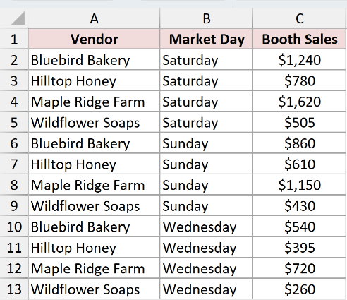
We want the vendors sorted by total booth sales, from largest to smallest.
Here is the formula:
=PIVOTBY(A2:A13,B2:B13,C2:C13,SUM,,,-2)
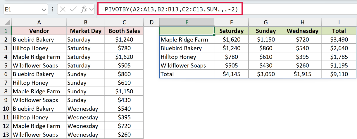
row_sort_order counts the row field first and the aggregated value second. A value of 2 sorts by each vendor’s total, and the minus sign makes the order descending.
The rows return Maple Ridge Farm at $3,490, Bluebird Bakery at $2,640, Hilltop Honey at $1,785, and Wildflower Soaps at $1,195.
The Total row stays at the bottom and shows $9,110 in I6.
Example 5: Filter Source Rows Inside PIVOTBY
Here’s how to summarize selected records without changing the source table.
Below is the dataset. It contains each server, meal period, order type, and ticket total in columns A through D.
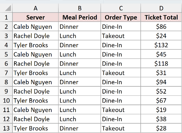
We want the meal-period totals for Dine-In orders only.
Here is the formula:
=PIVOTBY(A2:A13,B2:B13,D2:D13,SUM,,,,,,C2:C13="Dine-In")
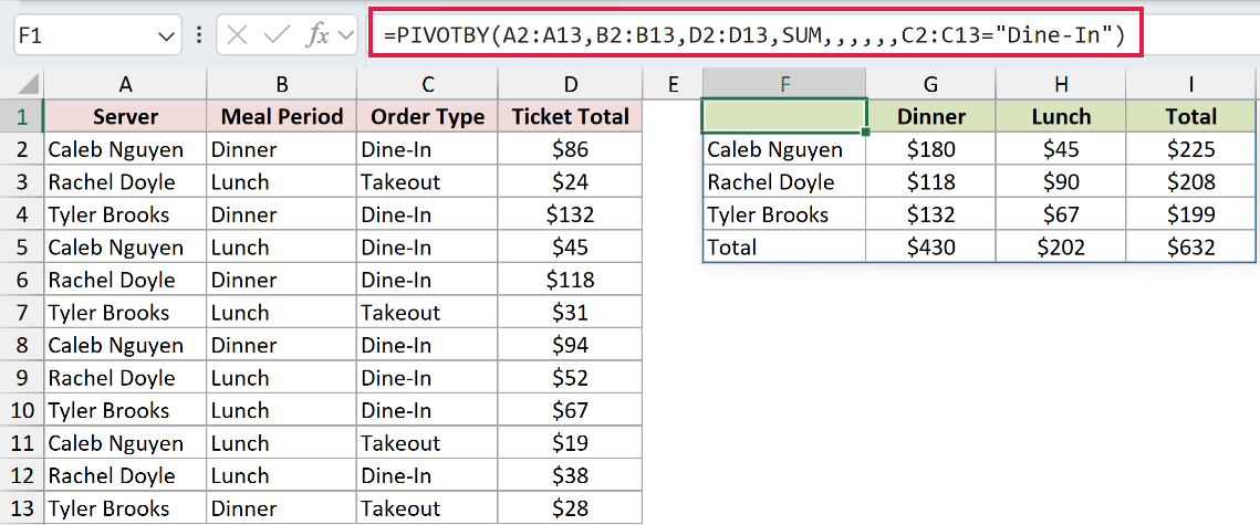
The test in the tenth argument returns TRUE for Dine-In rows. PIVOTBY keeps those rows and ignores the Takeout records without filtering the source range.
The six commas after SUM leave optional arguments five through nine empty before supplying filter_array.
Caleb Nguyen’s filtered total is $225, Rachel Doyle’s is $208, and Tyler Brooks’ is $199. The filtered grand total is $632.
Pro Tip: The filter array must have the same number of rows as the row and column field ranges. Mismatched range heights return #VALUE!.
Example 6: Calculate Percent of Grand Total
Finally, let’s show each intersection as a share of the complete dataset.
Below is the dataset. Column A lists insurance claim types, column B lists quarters, and column C contains claim amounts.
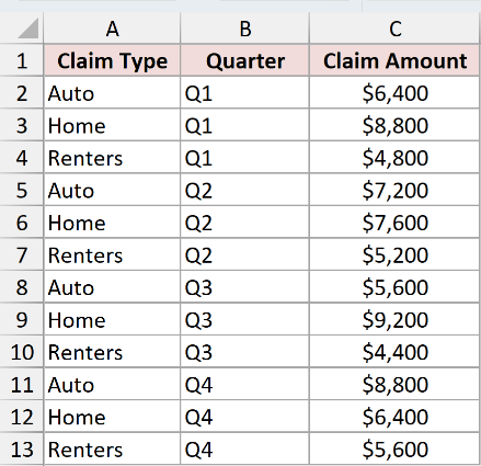
We want every claim amount displayed as a percentage of the grand total.
Here is the formula:
=PIVOTBY(A2:A13,B2:B13,C2:C13,PERCENTOF,,,,,,,2)
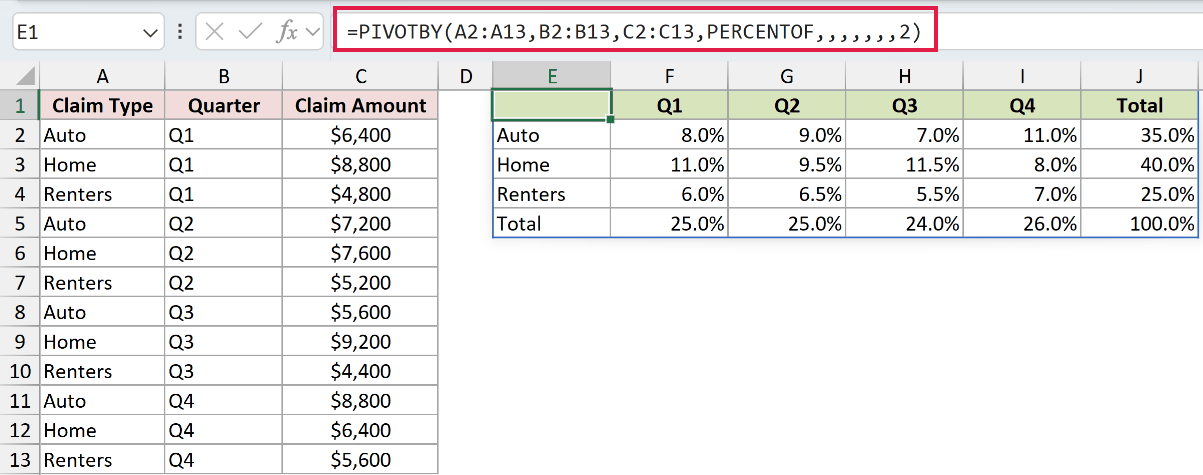
PERCENTOF changes the aggregation from an amount to a share. The relative_to value of 2 tells Excel to divide each result by the grand total.
The seven commas after PERCENTOF skip arguments five through ten before supplying relative_to.
Auto claims account for 35.0%, Home claims account for 40.0%, and Renters claims account for 25.0%. The bottom-right total in J5 is 100.0%.
For example, Home claims in Q3 return 11.5%, while the Q3 total across all claim types is 24.0%.
Tips & Common Mistakes
- PIVOTBY needs empty cells for its complete spill area, including the header row, row-label column, Total row, and Total column. Otherwise, Excel returns #SPILL!.
- All row fields, column fields, values, and filter arrays must have matching heights. Mismatched ranges return #VALUE!.
- row_total_depth controls horizontal total rows. col_total_depth controls vertical total columns. Each axis argument adds its matching Total row or Total column.
- An out-of-range sort number returns #VALUE!. Count row or column fields first, followed by value fields, when choosing row_sort_order or col_sort_order.
- PIVOTBY does not bring number formatting with it. Apply currency, percentage, or decimal formatting to the spilled output area.
- You can reference the complete spilled result elsewhere with the spill operator, such as
=E1#. - Use GROUPBY when you need a one-dimensional summary. For Excel 2021 or 2024, use a PivotTable or build a grid with UNIQUE and SUMIFS.
- PIVOTBY is formula-based and recalculates with its source. It cannot be dragged, filtered, or sliced through the PivotTable interface.
I’ve shown you how to build two-way totals and averages, remove Total rows and columns, and sort row groups by their totals.
We also filtered source rows and calculated percentages of the grand total. The blank corner cell is part of the spilled result, so leave it alone.
Related Excel Functions / Articles:
