How to Group Data in a Pivot Table (inc. Custom Groups)

Grouping data in an Excel PivotTable turns a long list into shorter, readable buckets, such as years and quarters, price bands, or regions.

The grouping stays inside the PivotTable, so your source data stays untouched.

I’ll show you how to group dates and numbers. You’ll also make custom text groups and use a helper column when the Group option isn’t available.

Method #1: Using the Group Feature for Dates

I use the Group feature when I want sales totals by year and quarter without listing every order date.

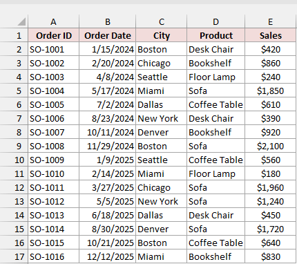
Below I have a dataset of furniture store orders with dates and sales amounts. I want to total sales by year and quarter.

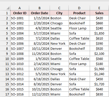
I start with a PivotTable that has Order Date in Rows and Sales in Values.

You can see all 16 dates under Row Labels, with Sum of Sales beside them and a Grand Total of $14,970.

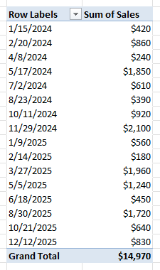
In Excel 2016 and later, including Microsoft 365, Excel may add Years and Quarters automatically when you add a date field.

It may also add Months; if you see plain dates like mine, use the steps below.

Let me show you how to group these dates into years and quarters.

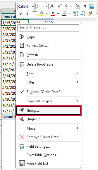
1. Right-click any date in the Row Labels column and click Group.

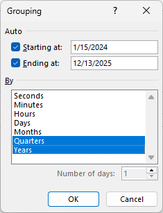
2. In the Grouping dialog, leave Starting at and Ending at as they are. Excel fills in the first and last date. In the By list, click Months to deselect it, then click Quarters and Years so both are selected. Click OK.

The PivotTable now groups quarters under each year, making it shorter.

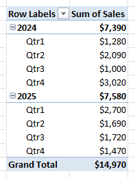
I get these totals for each year and its quarters.

• 2024 totals $7,390. Qtr1 is $1,280, Qtr2 is $2,090, Qtr3 is $1,000, and Qtr4 is $3,020.
• 2025 totals $7,580. Qtr1 is $2,700, Qtr2 is $1,690, Qtr3 is $1,720, and Qtr4 is $1,470.
• Grand Total is $14,970.

You can click the minus button next to a year to collapse its quarters and show the yearly total.

Note: If you select only Months for dates spanning multiple years, you put January 2024 and January 2025 in the same Jan group. Select Months and Years together to keep them apart.

Method #2: Using the Group Feature for Numbers

You can use the same Group feature to put numbers into bands instead of grouping dates.

Below I have a dataset of furniture store orders and sales amounts. I want to count orders in $500 bands, starting with 0-499.

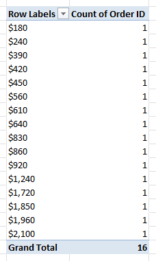
I start with a PivotTable that has Sales in Rows and Order ID in Values.

Because Order ID contains text, Excel counts the orders rather than adding the IDs. The header reads Count of Order ID.

You can see each sales amount on its own row with a count of 1, and a Grand Total of 16.

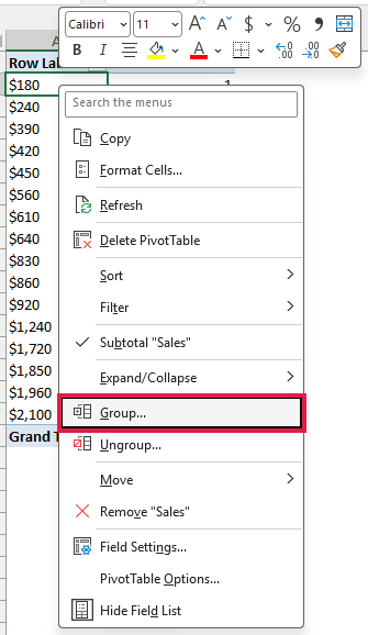
Let me show you how to turn these individual amounts into $500 bands.

1. Right-click any sales amount in the Row Labels column and click Group.

2. In the Grouping dialog, set Starting at to 0, Ending at to 2499, and By to 500. Click OK.

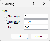
The PivotTable now shows one count for each sales band instead of a separate row for each amount.

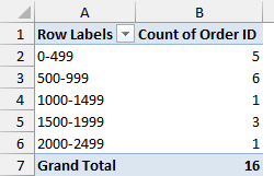
I get the following order counts.

• 0-499 has 5 orders.
• 500-999 has 6 orders.
• 1000-1499 has 1 order.
• 1500-1999 has 3 orders.
• 2000-2499 has 1 order.
• Grand Total is 16 orders.

You control the bands with the three settings in the Grouping dialog.

• With Starting at, you set the bottom of the first band.
• With By, you set the width of each band.
• With Ending at, you set where the last band stops.

Excel fills in the smallest and largest amounts, 180 and 2100, as the default limits. Without changing them, the first band would start at 180.

I’d replace these limits with round numbers so the bands read better.

Note: You won’t see a sales band in the PivotTable if it has no orders.

Method #3: Using Group Selection for Custom Groups

You can also choose which text items belong together and give each group your own name.

Below I have a dataset of furniture store orders from seven cities. I want to group the cities into three regions and compare their sales.

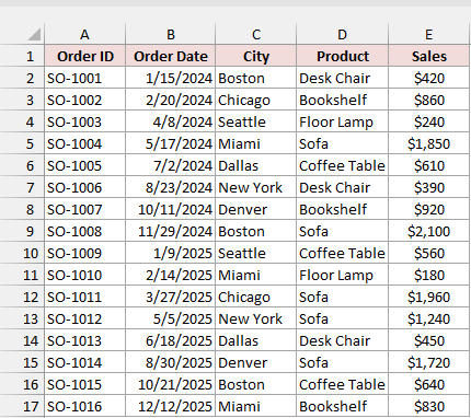
I start with a PivotTable that has City in Rows and Sales in Values. I haven’t added any regions to the source data.

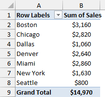
I get these city totals under Sum of Sales.

• Boston totals $3,160.
• Chicago totals $2,820.
• Dallas totals $1,060.
• Denver totals $2,640.
• Miami totals $2,860.
• New York totals $1,630.
• Seattle totals $800.
• Grand Total is $14,970.

Let me show you how to turn these city rows into regions.

1. Hold Ctrl and click Boston, Miami, and New York in the Row Labels column. Then right-click one of the selected cells and click Group.

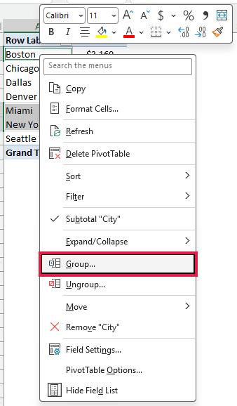
Excel puts the three cities under a new item called Group1, with a sales total of $7,650.

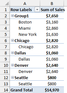
Each ungrouped city appears as a one-item group, such as a Chicago heading with Chicago underneath. Those duplicate headings disappear once you’ve grouped every city.

2. Click the Group1 cell, type East, and press Enter.

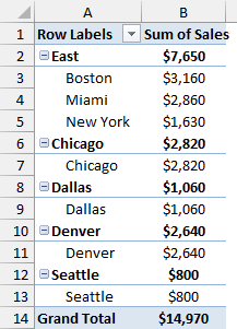
The group is now named East, with Boston, Miami, and New York underneath and a total of $7,650.

3. Select Chicago and Dallas, group them, and rename the group Central. Then select Denver and Seattle, group them, and rename the group West.

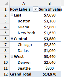
All seven cities now belong to their regions.

• East contains Boston, Miami, and New York, totaling $7,650.
• Central contains Chicago and Dallas, totaling $3,880.
• West contains Denver and Seattle, totaling $3,440.
• Grand Total is $14,970.

4. To see the region totals without the city rows, right-click any region name, go to Expand/Collapse, and click Collapse Entire Field.

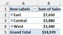
The collapsed PivotTable shows East at $7,650, Central at $3,880, and West at $3,440, with a Grand Total of $14,970.

Grouping also adds a new field named City2 to the PivotTable Fields list. You can rename it to Region using the steps in the FAQ.

You can use the Group Selection button on the PivotTable Analyze tab instead of the right-click menu, too.

Method #4: Using a Helper Column in the Source Data

You can keep the region assignments in your source data instead, so you can reuse them in other PivotTables.

I’d use a helper column when I need the same groups in several reports or someone else maintains the city-to-region mapping.

You can also use this approach when the Group option isn’t available, such as for custom groups in a PivotTable built on the Data Model.

Below I have furniture store orders with an empty Region column in F and a city-to-region lookup table in H1:I8. I want sales totals by region.

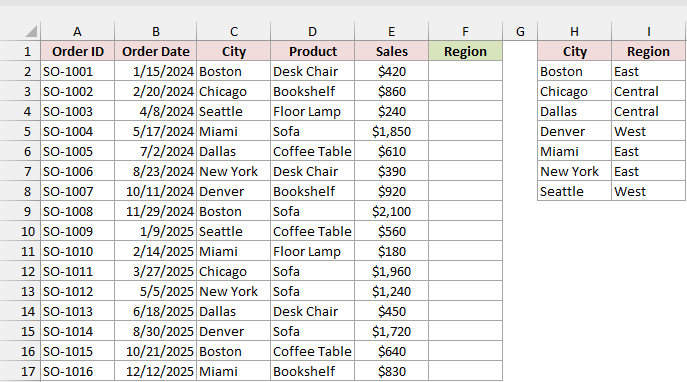
I use these assignments in the lookup table.

• Boston, Miami, and New York belong to East.
• Chicago and Dallas belong to Central.
• Denver and Seattle belong to West.

I enter this formula in F2 to return the region for each order.

=XLOOKUP(C2:C17,H2:H8,I2:I8)

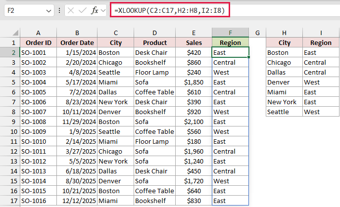
The formula spills down the column automatically, returning all 16 regions.

How does this formula work?

I use XLOOKUP to look up each city in C2:C17 in the lookup table’s City column, H2:H8.

I use it to return the matching region from I2:I8. Because I use a whole range as the lookup value, I get all 16 results from one formula.

If you’re using an Excel Table, enter =XLOOKUP(C2,$H$2:$H$8,$I$2:$I$8) as a regular formula instead, because you can’t use spilled formulas inside a Table.

You can now create a PivotTable from A1:F17, with Region in Rows and Sales in Values.

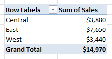
The PivotTable shows Central at $3,880, East at $7,650, and West at $3,440, with a Grand Total of $14,970.

The regions appear in alphabetical order here. You can reuse the groups in every PivotTable built from this data because they’re stored in the source.

How to Ungroup Data in a Pivot Table

You can undo grouping when you want to see the original items again.

1. Right-click any grouped item, such as a year or quarter from Method #1 or a region from Method #3, and click Ungroup.

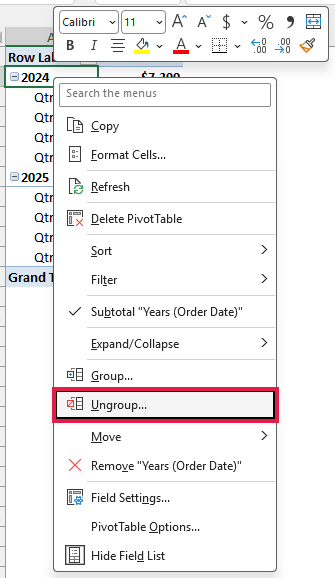
The PivotTable goes back to the original items. For custom groups, you can ungroup each group, or the City2 field, the same way.

Additional Notes About Grouping Data in a Pivot Table

You may need to account for these behaviors when grouping data in a PivotTable.

• PivotTables built from the same source share a PivotCache. Grouping dates or numbers in one also groups that field in the others. For different groupings, give the second PivotTable its own source, such as another named range pointing to the same data, and build it from that name.
• “Cannot group that selection” usually appears when your date or number column has blanks or values stored as text. Fix the source data, refresh the PivotTable, and try again.
• You can turn off automatic date grouping through File > Options > Data. Check “Disable automatic grouping of Date/Time columns in PivotTables”.
• You can group dates in a Data Model PivotTable, but you can’t group numbers into ranges or create custom groups there. Use a helper column, as in Method #4.
• Excel doesn’t automatically add a new city to a custom group when you refresh. It appears on its own until you group it.

Frequently Asked Questions

Let me answer a few questions you might have when setting up your groups.

How Do I Group Dates by Week in a Pivot Table?

You can select only Days in the Grouping dialog and set Number of days to 7.

You should also set Starting at to a Monday, or whichever day you want your week to start.

How Do I Rename the City2 Field Created by Custom Grouping?

You can click any region in the PivotTable, then go to the PivotTable Analyze tab and type Region in the Active Field box. Press Enter.

You can also right-click a region, open Field Settings, and change Custom Name to Region.

Why Is the Group Option Greyed Out?

The most common cause is a PivotTable built on the Data Model, which doesn’t support number or custom grouping.

You can use a helper column to put the groups in your source data instead.

Does Grouping Change My Source Data?

No, grouping only changes how the PivotTable displays your data. The original rows in your dataset stay the same.

Conclusion

I’d start with Group for dates and numbers, since you can set up the buckets in a few clicks.

I’d use Group Selection when you want to choose your own text groups.

If you need groups you can reuse, I’d keep them in a helper column, which also works with the Data Model.

Other Excel articles you may also like:

• How to Group by Months in Excel Pivot Table?
• How to Use a Timeline in a PivotTable in Excel
• Reorder Rows in Pivot Table in Excel
• Pivot Table vs Pivot Chart in Excel
• GROUPBY Function in Excel
• PIVOTBY Function in Excel
• How to Add a Calculated Item to Pivot Table in Excel