
Excel’s CODE function returns the numeric character code for the first character in a text value.
It can help inspect an unexpected leading character or distinguish characters that look similar. The result depends on the character set used by the computer.
For Unicode code points, use UNICODE instead.
In this article, I’ll show you how to identify character codes, detect hidden nonbreaking spaces, and test whether text starts with an uppercase letter.
CODE Function Syntax in Excel
The CODE function takes one text value and returns the system code page value for its first character.
=CODE(text)
- text (required) is the text whose first character you want to examine. It can be typed directly or supplied through a cell reference.
When to Use CODE Function
- Identify an invisible or unexpected character at the beginning of imported text.
- Compare the codes for uppercase letters, lowercase letters, digits, and symbols.
- Check whether text begins with a letter from a specific code range.
- Convert a character to a number before using that number in another calculation.
- Pair CODE with CHAR to inspect and rebuild characters on the system code page.
Example 1: Get the Code of the First Character
Let’s start with a simple rule. CODE reads only the first character.
Below is the dataset. It compares the single character A with the full text entry Ashland Supply Co.

We want to find the code returned for each entry.
Here is the formula for the single character:
=CODE(B1)

And here is the formula for the full text entry:
=CODE(B2)

Both formulas return 65 because both entries begin with uppercase A. Everything after that first character is ignored.
To inspect a different position, first extract that character with a function such as MID or RIGHT, then pass the extracted character to CODE.
Example 2: Get Character Codes for a Column
Now let’s check several helpdesk status flags at once.
Below is the dataset. Column A contains ticket IDs, and column B contains uppercase letters, lowercase letters, and symbols used as status flags.
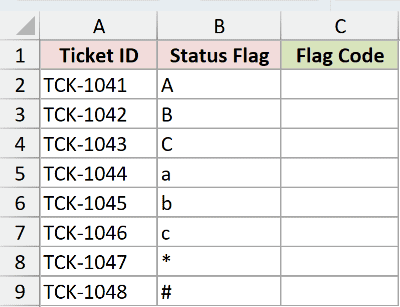
We want one formula to return the code for every flag in column B.
Here is the formula:
=CODE(B2:B9)
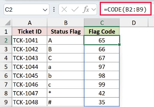
The formula spills eight results into C2:C9. Uppercase A, B, and C return 65, 66, and 67.
Lowercase a, b, and c return 97, 98, and 99. The asterisk returns 42, while the hash symbol returns 35.
Case matters here. Each lowercase English letter has a code 32 higher than its uppercase version.
Pro Tip: Keep the cells below the formula empty. Existing content in the spill range causes a #SPILL! error.
Example 3: Find a Hidden Non-Breaking Space
Here’s a frustrating problem you may meet after pasting names from a web report.
Below is the dataset. Column A contains eight customer names, and four begin with an invisible non-breaking space.
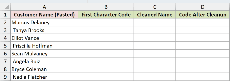
We want to identify the hidden character, remove it, and verify that each cleaned name now begins with its visible first letter.
First, use CODE to inspect the first character in every pasted name:
=CODE(A2:A9)
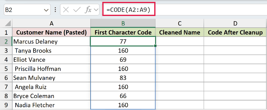
On Windows, the affected rows return 160. The clean rows return the codes for M, E, S, and B: 77, 69, 83, and 66.
TRIM removes the ordinary space character, which has code 32. It does not remove a non-breaking space with code 160.
CLEAN does not help here because it removes only codes 0 through 31.
Next, remove character 160 from every name:
=SUBSTITUTE(A2:A9,CHAR(160),"")
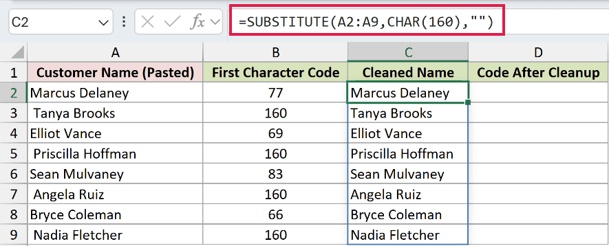
SUBSTITUTE removes the non-breaking space where it exists and leaves the other names unchanged.
Finally, run CODE against the cleaned names:
=CODE(C2:C9)
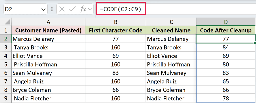
The cleaned names now return 77, 84, 69, 80, 83, 65, 66, and 78. Those are the codes for their visible first letters.
Pro Tip: Codes above 127 can differ between Windows and Mac. Use UNICHAR(160) to create a platform-safe non-breaking space.
Example 4: Convert Symbols With CODE and CHAR
Next, let’s turn a set of report symbols into numbers and then rebuild them.
Below is the dataset. Column A contains eight legend symbols, including punctuation marks and three extended characters.
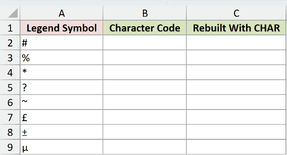
We want to get each symbol’s code and confirm that CHAR can return the original symbol.
First, get the code for each symbol:
=CODE(A2:A9)
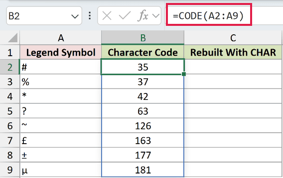
The hash, percent, asterisk, question mark, and tilde return 35, 37, 42, 63, and 126.
On Windows, the pound, plus-minus, and micro symbols return 163, 177, and 181.
Now pass those codes to CHAR:
=CHAR(B2:B9)
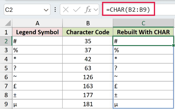
CHAR rebuilds the same eight symbols in column C. This shows how CODE and CHAR work as an inverse pair for supported system characters.
UNICODE and UNICHAR are the better pair when your text can contain characters outside the system code page. UNICODE returns a true Unicode code point.
Example 5: Check for an Uppercase First Letter
Finally, let’s classify product names by their first character.
Below is the dataset. Column A contains product names beginning with uppercase letters, lowercase letters, or the digit 4.
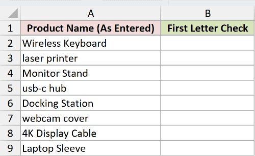
We want to label each entry as Uppercase, Lowercase, or Not a letter.
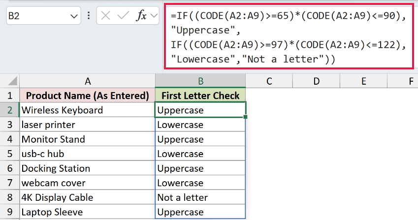
Here is the formula:
=IF((CODE(A2:A9)>=65)*(CODE(A2:A9)<=90),"Uppercase",IF((CODE(A2:A9)>=97)*(CODE(A2:A9)<=122),"Lowercase","Not a letter"))
How this formula works:
- The first two comparisons test whether the code falls from 65 through 90, the range for uppercase English letters.
- Multiplication evaluates both comparisons row by row. AND would collapse the arrays to one result and stop the formula from spilling correctly.
- The nested IF then checks codes 97 through 122 for lowercase English letters.
- Any remaining code returns Not a letter. That is why 4K Display Cable gets the third label.
The results classify Wireless Keyboard, Monitor Stand, Docking Station, and Laptop Sleeve as Uppercase. The three lowercase entries are labeled Lowercase.
In Excel 365, REGEXTEST offers a shorter way to check whether text begins with an uppercase letter. The CODE approach still works in older Excel versions.
Tips & Common Mistakes
- CODE returns the code for the first character only. It does not evaluate the whole text string.
- CODE returns a number, not text, so you can compare, sort, or use the result in arithmetic.
- CODE uses your computer’s system code page. On Windows this is ANSI, while codes above 127 can differ on a Mac.
- On Windows, CODE and UNICODE agree for basic ASCII characters and code values 160 through 255. Between 128 and 159, they can differ. For example, the euro sign returns 128 with CODE and 8364 with UNICODE.
- Blank cells and empty text strings return #VALUE!. Check for empty inputs before passing them to CODE.
- Numbers are converted to text first. A multi-digit number returns the code of its first digit, not the original number.
- A range-based CODE formula spills in Excel 2021, Excel 2024, Microsoft 365, and Excel for the web. In Excel 2019 and earlier, enter the formula one row at a time.
- If Excel applies implicit intersection, CODE returns one result instead of spilling the full range.
- Avoid treating CODE as a complete Unicode tool. Use UNICODE when text may include symbols or characters outside your system code page.
CODE is handy when the first character matters, especially when that character is invisible or must be tested numerically.
For text beyond the system code page, choose UNICODE so the returned number is a true Unicode code point.
Related Excel Functions / Articles:
