
Excel’s ACCRINT function returns the interest accrued on a coupon-paying security between the issue date you provide and its settlement date.
For a bond bought between coupon dates, this amount is added to the quoted clean price to determine what the buyer pays at settlement.
In this article, I’ll show you how to calculate accrued interest, avoid an original-issue-date trap, build a month-end schedule, and compare day-count bases.
ACCRINT Function Syntax in Excel
The ACCRINT function uses the security’s dates, coupon rate, face amount, payment frequency, and day-count convention.
=ACCRINT(issue, first_interest, settlement, rate, par, frequency, [basis], [calc_method])
- issue (required) is the security’s issue date, or the previous coupon date when calculating the current coupon period.
- first_interest (required) is the first interest date, or the next coupon date when calculating the current coupon period.
- settlement (required) is the date the buyer takes ownership of the security.
- rate (required) is the security’s annual coupon rate.
- par (required) is the face amount you bought. If omitted, Excel uses $1,000.
- frequency (required) is 1 for annual, 2 for semiannual, or 4 for quarterly coupon payments.
- basis (optional) sets the day-count convention. Omitting basis uses 0 (US (NASD) 30/360). Use 1 for actual/actual, 2 for actual/360, 3 for actual/365, or 4 for European 30/360.
- calc_method (optional) matters only when settlement is later than first_interest. TRUE or an omitted value returns total accrued interest from issue to settlement. FALSE returns accrued interest from first_interest to settlement.
When to Use ACCRINT Function
- Calculate accrued interest when buying or selling a bond between coupon dates.
- Add accrued interest to a clean bond price to find the full settlement amount.
- Record accrued interest receivable at each month end.
- Compare results under different market day-count conventions.
- Calculate current-period accruals across a list of bond trades.
Example 1: Calculate Interest Before First Coupon
Let’s start with a bond bought before its first coupon payment.
Below is the dataset. The card lists the issue, first interest, and settlement dates, plus the coupon terms. Empty bordered result cell B8 sits beside A8’s bold “Accrued Interest” label.
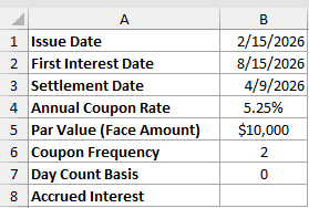
We want to calculate the interest earned from the February 15 issue date through the April 9 settlement date.
Here is the formula:
=ACCRINT(B1,B2,B3,B4,B5,B6,B7)
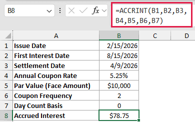
The formula returns $78.75 on a $10,000 face amount with a 5.25% annual coupon and semiannual payments.
Basis 0 applies the US 30/360 convention. For these dates, Excel counts 54 accrued days.
Example 2: Avoid the Original Issue Date Trap
Here’s the common mistake that produces an unexpectedly large result on an older bond.
Below is the dataset. It includes the original issue date, first interest date, last and next coupon dates, settlement date, and bond terms.
The two bordered result cells are empty.
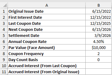
We want the interest accrued since the most recent coupon, then we’ll compare it with a formula using the original issue date.
Here is the current-period formula:
=ACCRINT(B3,B4,B5,B6,B7,B8,B9)
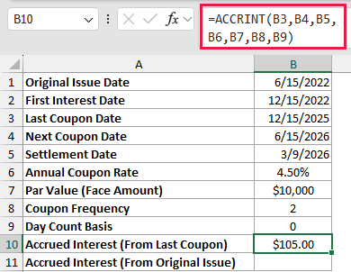
Now compare it with the formula that uses the bond’s original issue and first interest dates:
=ACCRINT(B1,B2,B5,B6,B7,B8,B9)
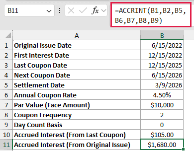
The current-period formula returns $105.00 because it starts at the December 15, 2025 coupon date.
The original-date formula returns $1,680.00. ACCRINT counts from whatever you pass as issue, so it includes interest accumulated since June 15, 2022.
For a bond bought after its first coupon, pass the last coupon date as issue and the next coupon date as first_interest.
Example 3: Calculate Accrued Interest for Multiple Bonds
Now let’s calculate current-period interest across several bond trades.
Below is the dataset. Each row lists a bond, maturity, settlement, coupon rate, face amount, and frequency. The green Accrued Interest column contains empty bordered cells.
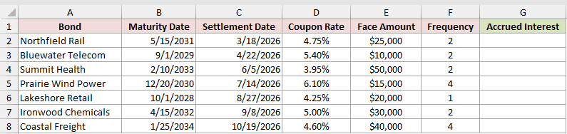
We want each row to find its surrounding coupon dates and return the interest accrued through settlement.
Here is the formula entered in G2 and copied down:
=ACCRINT(COUPPCD(C2,B2,F2,0),COUPNCD(C2,B2,F2,0),C2,D2,E2,F2,0)
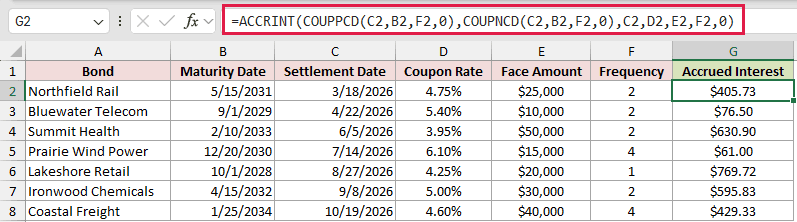
COUPPCD returns the last coupon date before each row’s settlement date. COUPNCD returns the next coupon date after it.
Both use the maturity date and frequency to set the coupon schedule.
Those dates become ACCRINT’s issue and first_interest arguments. The Northfield Rail row returns $405.73.
The formula is filled down because ACCRINT returns one #VALUE! when given a plain range instead of one bond’s inputs.
Pro Tip: In Excel 2021, Excel 2024, and Microsoft 365, adding +0 to a range passed directly into an ACCRINT argument, such as rate, can coerce a spill. Fill-down remains the default for this nested trade-list formula.
Example 4: Calculate a Bond’s Full Settlement Amount
Let’s use accrued interest to find the total a bond buyer pays at settlement.
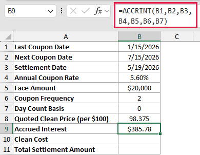
Below is the dataset. The card includes the coupon dates, settlement date, bond terms, and quoted clean price per $100. All three bordered result cells are empty.
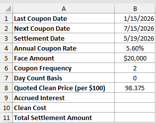
We want to calculate accrued interest, convert the clean quote into a holding cost, and add both amounts.
First, calculate the interest accrued since the last coupon date:
=ACCRINT(B1,B2,B3,B4,B5,B6,B7)
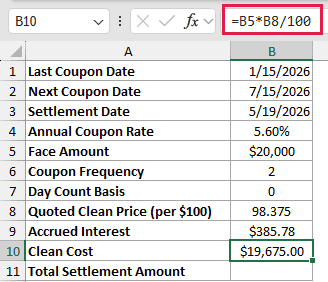
Next, calculate the clean cost from the face amount and quoted price:
=B5*B8/100
Finally, add the accrued interest to the clean cost:
=B10+B9
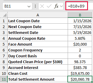
ACCRINT returns $385.78. The clean quote converts to $19,675.00 for the $20,000 face amount.
Adding them produces a total settlement amount of $20,060.78. This full amount is sometimes called the dirty price.
Example 5: Build a Month-End Accrual Schedule
Here’s an accounting example that tracks accrued interest throughout the year.
Below is the dataset. Column A lists 2026 month ends, with empty bordered cells under column B’s green header. The card in columns D and E contains the bond inputs.
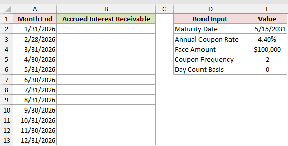
We want to calculate the accrued interest receivable at every month end.
Here is the formula entered in B2 and copied down:
=ACCRINT(COUPPCD(A2,$E$2,$E$5,$E$6),COUPNCD(A2,$E$2,$E$5,$E$6),A2,$E$3,$E$4,$E$5,$E$6)
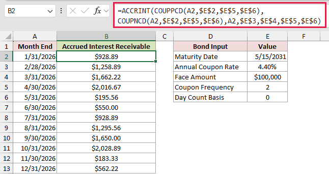
COUPPCD and COUPNCD find the coupon dates surrounding each month end. ACCRINT treats that month end as the settlement date.
The receivable rises to $2,016.67 by April 30, then falls to $195.56 on May 31 after the May 15 coupon.
It resets again after the November 15 coupon because a new coupon period has started.
Example 6: Compare Day Count Basis Results
The last example shows why the basis argument matters.
Below is the dataset. It lists five basis codes, their day-count conventions, and typical uses. Empty bordered result cells sit under a green header beside the right-side bond-input card.
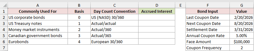
We want to calculate the same bond’s accrued interest under each day-count basis.
Here is the formula entered in D2 and copied down:
=ACCRINT($G$2,$G$3,$G$4,$G$5,$G$6,$G$7,B2)
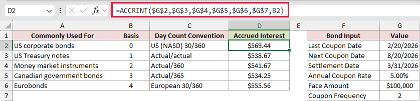
The absolute references keep the bond inputs fixed, while the relative B2 reference changes for each basis row.
- Basis 0, US 30/360, returns $569.44.
- Basis 1, actual/actual, returns $538.67.
- Basis 2, actual/360, returns $541.67.
- Basis 3, actual/365, returns $534.25.
- Basis 4, European 30/360, returns $555.56.
The dates cross February and settle on March 31, so the conventions count or scale the accrued period differently.
The “Commonly Used For” labels describe typical conventions. Use the basis specified in the security’s documentation.
Tips & Common Mistakes
- ACCRINT does not natively spill across a plain range. Use one formula per bond and copy it down.
- Omitting par makes Excel calculate interest for a $1,000 face amount.
- Frequency accepts only 1, 2, or 4. A value such as 3 returns #NUM!.
- The issue date must be earlier than settlement. An equal or later issue date returns #NUM!.
- Enter valid Excel dates. Invalid date text returns #VALUE!.
- Microsoft defines calc_method FALSE as starting at first_interest.
- Use ACCRINTM for securities that pay interest only at maturity, rather than through periodic coupons.
ACCRINT handles the interest that builds up between coupon dates, as long as you map each date and basis correctly.
For older bonds, use the previous and next coupon dates so the result covers the current coupon period.
Other Excel articles you may also like:
