
SUMIFS is a useful function when you want to add up values that meet one or more conditions, like sales for the West region.
It works fine when the numbers you’re adding sit in one column. But monthly data usually runs sideways, with a column for each month.
The catch is that SUMIFS can’t pick a column by its header. INDEX MATCH can, and it hands the right month straight to SUMIFS.
In this article, I’ll show you six ways to do it, including a second condition, the SUMIF version, XLOOKUP, and SUMPRODUCT.
Method #1: Using SUMIFS With INDEX and MATCH
This is the method I recommend for most people. It works in Excel 2007 and later, and you can add more conditions later.
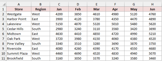
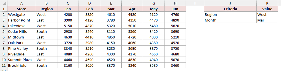
Below I have a dataset with store sales from January through June. I want to total March sales for stores in the West region.
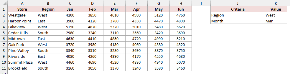
The criteria card has West in cell K2 and Mar in cell K3. Changing either value gives me a different regional or monthly total.
Here is the formula:
=SUMIFS(INDEX(C2:H11,0,MATCH(K3,C1:H1,0)),B2:B11,K2)
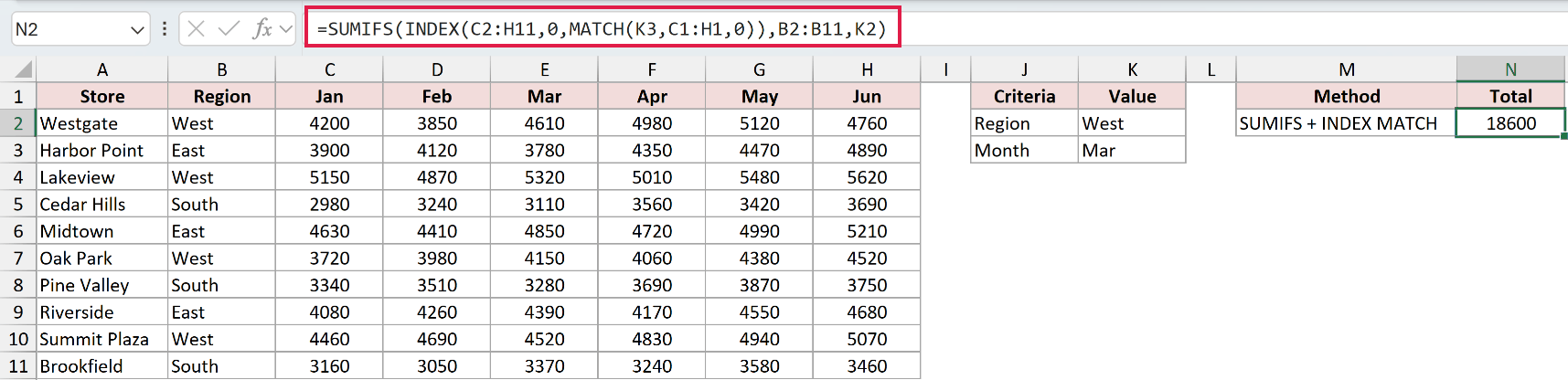
The formula returns 18,600, which is the total of 4,610, 5,320, 4,150, and 4,520 for the four West stores.
How does this formula work?
MATCH(K3,C1:H1,0) finds Mar in the header row and returns 3 because Mar is the third column within C1:H1.
INDEX(C2:H11,0,3) uses 0 for the row number, so it returns the entire March column from the sales data.
SUMIFS takes that column as its sum range. It checks B2:B11 for West and adds the matching March values.
Method #2: Using SUMIFS With Two Conditions
Here’s where SUMIFS earns its place. You can test the month column itself, so only the bigger stores count toward the total.
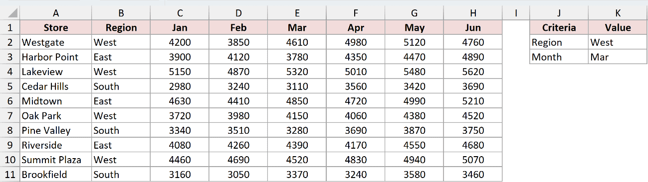
Below I have the same dataset. I want March sales for West stores, but only where that store sold more than 4,500.
Here is the formula:
=SUMIFS(INDEX(C2:H11,0,MATCH(K3,C1:H1,0)),B2:B11,K2,INDEX(C2:H11,0,MATCH(K3,C1:H1,0)),">4500")
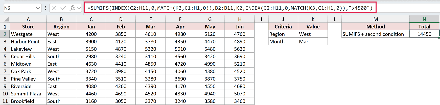
The formula returns 14,450. Oak Park’s 4,150 drops out, leaving 4,610, 5,320, and 4,520 in the total.
How does this formula work?
The INDEX MATCH part appears twice. The first one is the sum range, and the second one is the criteria range for the threshold.
That is the same March column doing two jobs. SUMIFS adds a value only when its row is West and the value clears 4,500.
Note: SUMIF cannot do this. It accepts one condition only, so a second test means switching to SUMIFS or SUMPRODUCT.
Method #3: Using SUMIF With INDEX and MATCH
SUMIF is the older, single-condition version of SUMIFS. It takes the criteria range first and the sum range last, which is the reverse order.
Reach for it when you have exactly one condition and prefer that argument order. Below I have the same store sales dataset.
Here is the formula:
=SUMIF(B2:B11,K2,INDEX(C2:H11,0,MATCH(K3,C1:H1,0)))
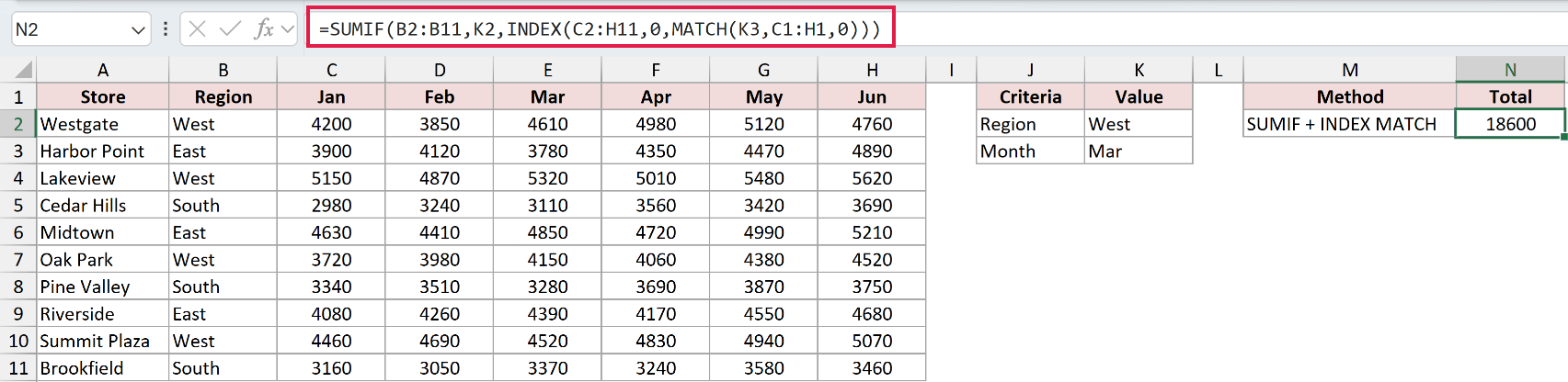
This formula also returns 18,600.
How does this formula work?
SUMIF checks B2:B11 for the region in K2, then adds the matching values from the March column returned by INDEX.
The INDEX MATCH part is identical to Method #1. Only its position changes, because SUMIF puts the sum range last.
Note: Keep the SUMIF criteria range and INDEX sum range aligned. If INDEX includes the header row, this example quietly returns 13,020 instead of 18,600.
Method #4: Using SUMIFS With XLOOKUP
If you use a newer version of Excel, XLOOKUP makes the column-selection part easier to read. It replaces both INDEX and MATCH.
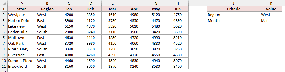
Below I have store sales by region and month. I want XLOOKUP to select March before SUMIFS totals the West rows.
Here is the formula:
=SUMIFS(XLOOKUP(K3,C1:H1,C2:H11),B2:B11,K2)
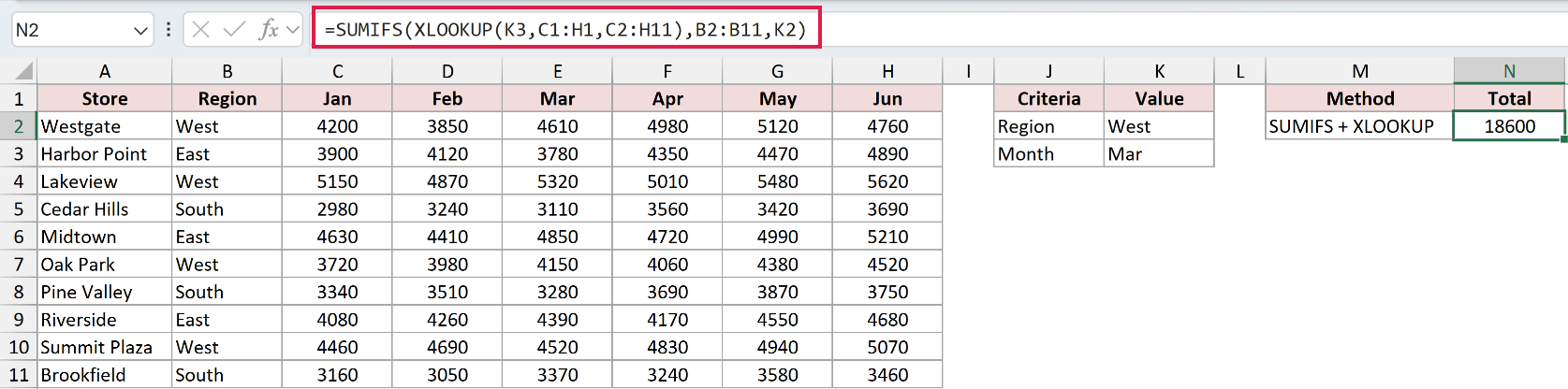
The result is 18,600.
How does this formula work?
XLOOKUP(K3,C1:H1,C2:H11) finds Mar in the headers and returns the corresponding values from the six-column sales area.
SUMIFS treats that returned March column as its sum range. It then adds only the values whose Region cells match West.
Note: XLOOKUP is available in Microsoft 365, Excel 2021, Excel 2024, and Excel for the web. Use an INDEX and MATCH method in older versions.
Method #5: Using the SUMPRODUCT Function
Here’s a formula that does not need INDEX. SUMPRODUCT can test the row labels and column headers together, then add where both match.
Below I have the six-month sales table. I want to total cells that sit in a West row and the Mar column.
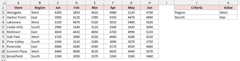
Here is the formula:
=SUMPRODUCT((B2:B11=K2)*(C1:H1=K3)*C2:H11)
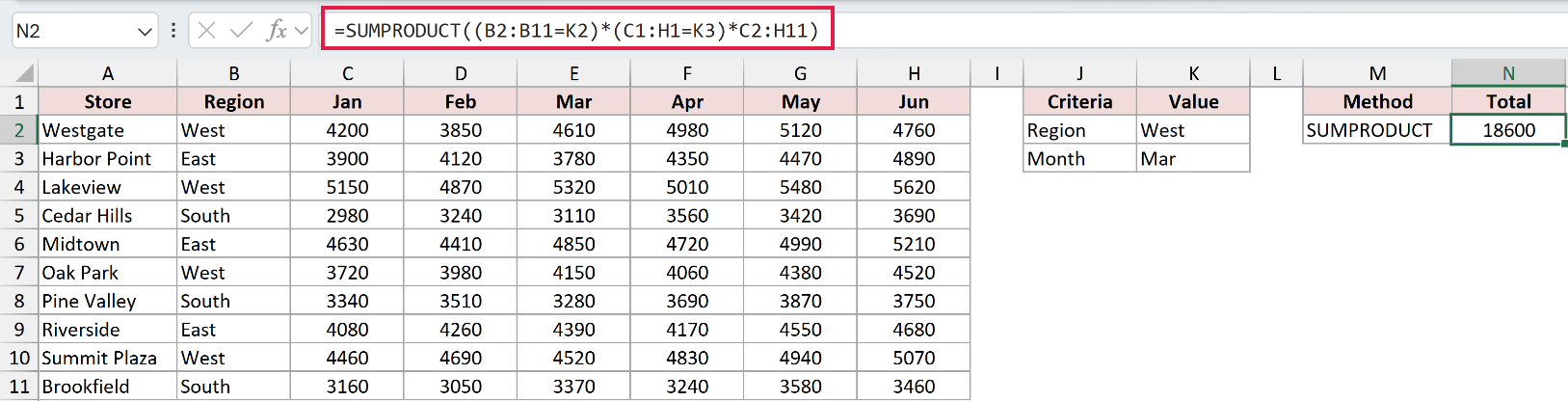
The formula returns 18,600 and works in Excel 2007 and later.
How does this formula work?
B2:B11=K2 creates a vertical set of TRUE and FALSE results for the selected region.
C1:H1=K3 creates a horizontal set for the selected month. Multiplication converts both sets to 1s and 0s across the grid.
SUMPRODUCT multiplies that grid by C2:H11. Only cells at the intersection of a matching row and column remain, and it adds those.
Method #6: Using SUMPRODUCT With INDEX:INDEX
This final method is useful when one selected month is not enough. It creates a range between two month columns and totals everything inside.
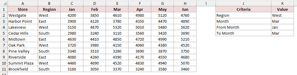
Below I have the same regional sales dataset. This time, I want to total West sales from January through March.
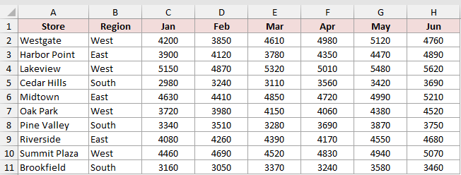
The criteria card has Jan in K4 and Mar in K5. Those cells define the first and last columns of the period.
Here is the formula:
=SUMPRODUCT((B2:B11=K2)*INDEX(C2:H11,0,MATCH(K4,C1:H1,0)):INDEX(C2:H11,0,MATCH(K5,C1:H1,0)))
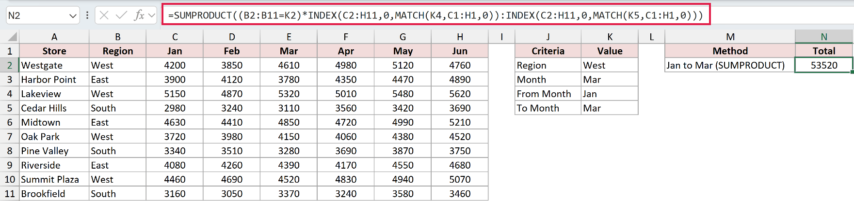
The result is 53,520 for the West stores from January through March.
How does this formula work?
The first INDEX and MATCH returns the January column reference. The second pair returns the March column reference.
The colon between those references creates the complete C2:E11 range, covering January, February, and March.
B2:B11=K2 identifies the West rows. SUMPRODUCT applies that test across all three month columns and adds the matches.
Note: SUMIFS cannot take a multi-column sum range like C2:E11 against B2:B11. It returns #VALUE!, so a month range needs SUMPRODUCT.
| Method | Works in | Best for |
|---|---|---|
| SUMIFS with INDEX and MATCH | Excel 2007 and later | A dependable formula that can accept more criteria |
| SUMIFS with two conditions | Excel 2007 and later | Filtering the month column itself as well as the region |
| SUMIF with INDEX and MATCH | Excel 2007 and later | A single condition with the classic SUMIF argument order |
| SUMIFS with XLOOKUP | Excel 2021 and later | A shorter, easier-to-read column lookup |
| SUMPRODUCT | Excel 2007 and later | Testing row and column conditions in one calculation |
| SUMPRODUCT with INDEX:INDEX | Excel 2007 and later | Summing a period between two selected month headers |
Additional Notes About Using SUMIFS With INDEX MATCH in Excel
- Keep the first and last data rows identical in every range. A mismatched header row makes SUMIFS return
#VALUE!, while SUMIF can silently return a wrong total. - SUMIFS puts the sum range first, SUMIF puts it last. Mixing up the two argument orders is the most common mistake here.
- Use 0 as MATCH’s final argument. Omitting it requests an approximate match, which is unreliable with unsorted month names.
- A trailing space in a header, such as
Mar, makes exact MATCH return#N/A. Correct the header or clean imported headers with TRIM. - SUMIFS cannot use a multi-column sum range such as C2:E11 with B2:B11. It returns
#VALUE!, so use SUMPRODUCT for a month range.
Frequently Asked Questions
Should I Use SUMIF or SUMIFS With INDEX MATCH?
Use SUMIFS. It does everything SUMIF does, accepts more conditions, and has shipped with Excel since 2007.
SUMIF is worth knowing because you will meet it in older workbooks, and its argument order is the reverse of SUMIFS.
Why Does My SUMIFS With INDEX MATCH Return #VALUE!?
The sum range and criteria range cover a different number of rows. That usually means INDEX included the header row and the criteria range did not.
Start both ranges on row 2 and end them on the same row, and the error clears.
How Do I Sum a Whole Row Matched by INDEX MATCH?
Use MATCH to find the store’s row, pass 0 as INDEX’s column number, and wrap the returned row in SUM.
For this dataset, the data array would be C2:H11 and the store names would be matched against A2:A11.
Do SUMIFS and INDEX MATCH Require Ctrl + Shift + Enter?
No. These formulas can be entered normally because INDEX returns a range reference that SUMIFS or SUMIF can use directly.
Can I Use Drop-Down Lists for the Region and Month?
Yes. Data Validation lists can supply K2 and K3, while the formulas stay unchanged. This helps prevent spelling differences and accidental spaces in criteria cells.
Conclusion
INDEX MATCH lets SUMIFS total a column chosen by its header. I recommend SUMIFS with INDEX and MATCH because it is dependable and easy to extend.
Use SUMIF only when you have one condition and prefer its argument order, and SUMPRODUCT for a range of months.
Other Excel articles you may also like:
