How to Count Words in Excel (in a Cell or Range)

If you want to know how many words are in a cell, Excel won’t tell you the way Word does. There’s no word count button and no WORDCOUNT function.

What you can do is count the spaces between the words and add one. That works well, as long as you deal with the things that throw the count off.

Extra spaces make the count too high. An empty cell returns 1 instead of 0. And text pasted from a web page often has spaces that aren’t really spaces.

In this article, I’ll show you six ways to count words, using LEN with SUBSTITUTE, TEXTSPLIT, SUMPRODUCT for a whole range, Power Query, and a short VBA function.

Method #1: Using LEN, TRIM, and SUBSTITUTE

This is the formula I reach for first. It counts the spaces between words and adds one, and it works in every version of Excel.

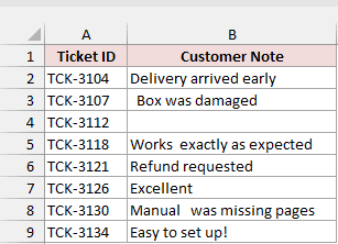
Below I have a list of support tickets with the customer’s note in column B. Some notes have extra spaces, and ticket TCK-3112 has no note at all.

I want the word count of each note in column C.

Here is the formula that counts the words in every note:

=IF(TRIM(B2:B9)="",0,LEN(TRIM(B2:B9))-LEN(SUBSTITUTE(TRIM(B2:B9)," ",""))+1)

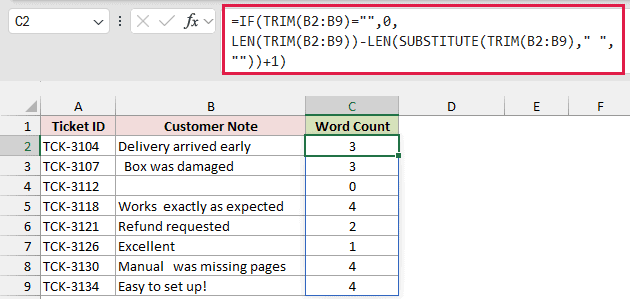
Enter it in C2 and it spills down the column automatically, one count for each note.

This spilling version needs Excel 2021 or Microsoft 365. In Excel 2019 or older, use B2 instead of B2:B9 in the formula, then copy it down to C9.

How does this formula work?

TRIM removes the spaces at the start and end of each note, and turns any run of spaces between words into a single space.

LEN(TRIM(B2:B9)) returns the length of the cleaned note. For “Delivery arrived early”, that’s 22 characters.

SUBSTITUTE(TRIM(B2:B9),” “,””) removes every space, and LEN returns the length of what’s left. That’s 20 for the same note.

The difference between the two lengths (22 – 20 = 2) is the number of spaces between words.

There’s always one more word than there are spaces, so the formula adds 1 to get 3.

The IF part checks whether the note is empty after trimming. If it is, the formula returns 0. Without it, TCK-3112 would show 1 word.

You may have seen a shorter version of this formula that skips TRIM. Here it is next to ours, so you can see what TRIM is doing:

=LEN(B2:B9)-LEN(SUBSTITUTE(B2:B9," ",""))+1

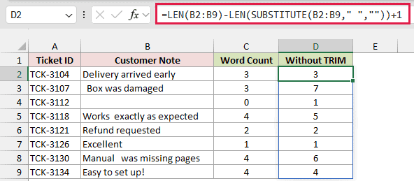
It gets the clean notes right, but every extra space counts as another word.

TCK-3107 has spaces around the text and shows 7 words instead of 3, and the empty note shows 1.

Note: Always keep TRIM in a word count formula unless you’re sure your text has exactly one space between words and none at the ends.

Method #2: Using the TEXTSPLIT Function

If you have Microsoft 365 or Excel 2024, TEXTSPLIT gives you a formula that reads almost like plain English. It splits the note into separate words, and COUNTA counts them.

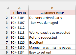
Below I have the same support tickets with the customer notes in column B. I want the number of words in each note in column C.

Here is the formula I entered in C2 and then copied down to C9:

=IF(TRIM(B2)="",0,COUNTA(TEXTSPLIT(TRIM(B2)," ")))

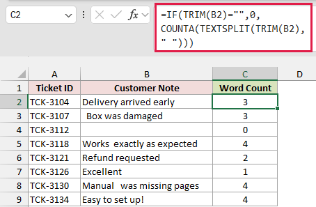
I’m using B2 and copying the formula down here. TEXTSPLIT can’t return a separate word list for every row of a range, so it works one cell at a time.

How does this formula work?

TRIM(B2) cleans up the extra spaces first, so there’s exactly one space between each pair of words.

TEXTSPLIT(TRIM(B2),” “) splits the cleaned note at every space. “Delivery arrived early” becomes three separate values: Delivery, arrived, and early.

COUNTA counts those values and returns 3.

The IF part returns 0 for an empty note. Without it, TEXTSPLIT would return a #VALUE! error for TCK-3112, and COUNTA would count that error as 1.

Note: TEXTSPLIT is only available in Microsoft 365, Excel 2024, and Excel for the web. In older versions, this formula returns a #NAME? error, so use Method #1 instead.

Method #3: Using SUMPRODUCT for a Range

Sometimes you don’t need a count for each cell. You just want the total number of words in a whole range, in one cell, without a helper column.

Below I have the same eight customer notes in B2:B9. I want the total word count in cell B11.

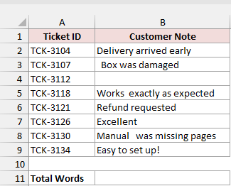
Here is the formula that returns the total:

=SUMPRODUCT(LEN(TRIM(B2:B9))-LEN(SUBSTITUTE(TRIM(B2:B9)," ",""))+(TRIM(B2:B9)<>""))

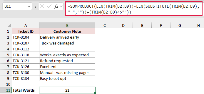
The formula returns 21, which is the sum of the counts you got in Method #1.

How does this formula work?

LEN(TRIM(B2:B9))-LEN(SUBSTITUTE(TRIM(B2:B9),” “,””)) is the same space count as in Method #1, done for all eight notes at once.

Instead of adding 1 with an IF, this formula adds (TRIM(B2:B9)<>””). That part returns TRUE for a note with text and FALSE for an empty one.

When Excel adds TRUE or FALSE to a number, it treats TRUE as 1 and FALSE as 0.

So every note with text gets its extra 1, and the empty note gets nothing.

SUMPRODUCT then adds up the eight counts and returns 21.

I’m not using IF here on purpose. In Excel 2019 and older, an IF inside SUMPRODUCT only works if you confirm the formula with Ctrl + Shift + Enter.

This version works in every version when you just press Enter.

Method #4: Using LET to Clean Line Breaks and Web Spaces

The formulas so far split words at regular spaces. Two other characters can sit between words and look just like a space: a line break and a nonbreaking space.

A line break is what you get when you press Alt + Enter in a cell. A nonbreaking space often comes along when you copy text from a web page.

Below I have the same ticket notes with two more rows. TCK-3139 has a line break between “Label” and “was”, and TCK-3143 has a nonbreaking space between “link” and “not”.

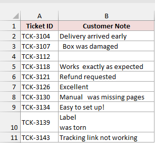
Here is the formula that swaps both characters for regular spaces before counting:

=LET(t,TRIM(SUBSTITUTE(SUBSTITUTE(B2:B11,CHAR(160)," "),CHAR(10)," ")),IF(t="",0,LEN(t)-LEN(SUBSTITUTE(t," ",""))+1))

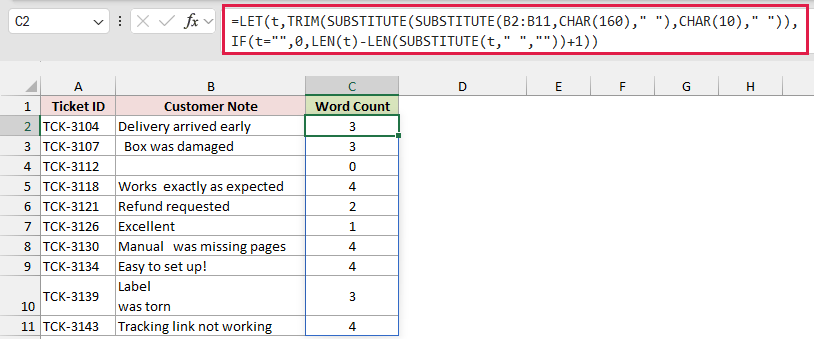
Enter it in C2 and it spills down to C11. TCK-3139 shows 3 words and TCK-3143 shows 4, which are the right counts.

How does this formula work?

CHAR(160) is the nonbreaking space, and CHAR(10) is the line break. The two SUBSTITUTE functions replace each of them with a regular space.

TRIM then cleans up any extra spaces, and LET stores the cleaned text under the name t.

That way the formula doesn’t have to repeat the whole cleaning part three times.

The rest is the same formula as Method #1, just using t instead of TRIM(B2:B9).

Here’s the Method #1 formula on the same ten notes, so you can see why the cleaning step matters:

=IF(TRIM(B2:B11)="",0,LEN(TRIM(B2:B11))-LEN(SUBSTITUTE(TRIM(B2:B11)," ",""))+1)

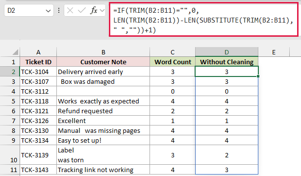
It returns 2 for TCK-3139 and 3 for TCK-3143, one word short on each. The other eight notes match, because they only use regular spaces.

Note: LET needs Excel 2021 or Microsoft 365. In older versions, put the cleaning part in place of each t, use B2 instead of B2:B11, and copy the formula down.

Method #5: Using Power Query

If you get a new batch of notes every week, Power Query lets you set up the word count once. After that, you refresh the query and the counts update.

Below I have the eight support tickets with the customer notes in column B. I want a new table with a Word Count column next to each note.

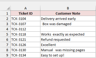
Here are the steps to count words with Power Query:

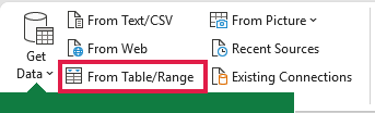
1. Select any cell in the dataset, then on the Data tab, click From Table/Range.

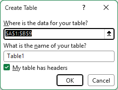
2. In the Create Table dialog box, make sure the range is right and My table has headers is checked, then click OK. Power Query needs the data in an Excel Table, and this step creates one.

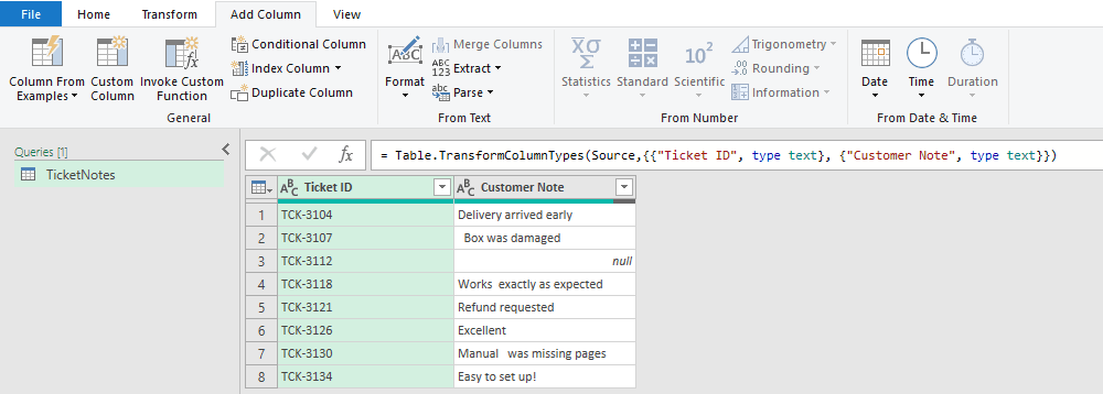
3. The Power Query Editor opens. On its Add Column tab, click Custom Column.

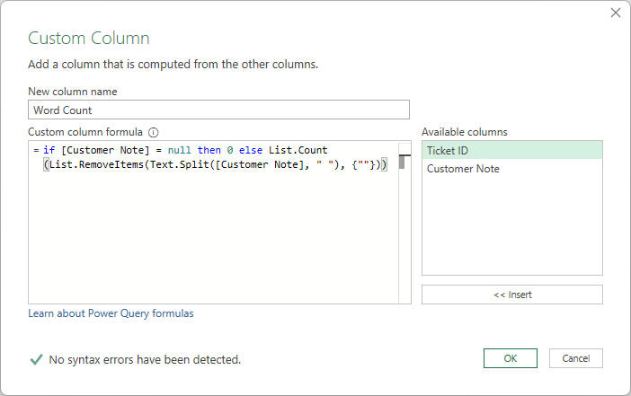
4. In the Custom Column dialog box, type Word Count as the new column name, enter the formula below, and click OK.

if [Customer Note] = null then 0 else List.Count(List.RemoveItems(Text.Split([Customer Note], " "), {""}))

Power Query adds the Word Count column to the preview, with one count for each note.

5. On the Home tab of the Power Query Editor, click Close & Load.

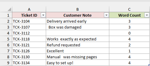
Power Query loads the result as a new table on a new sheet, with the Word Count column next to the notes. The counts match Method #1.

How does this formula work?

Text.Split([Customer Note], ” “) splits the note at every space. Extra spaces leave empty pieces behind, so List.RemoveItems removes every empty piece (“”) from the list.

List.Count then counts the words that are left.

The if part handles the empty note. An empty cell comes into Power Query as null, and the formula returns 0 for it.

Note: The loaded table doesn’t update on its own. When you add or change notes, go to Data and click Refresh All to update the counts.

Method #6: Using a VBA Custom Function

If you count words a lot, you can build your own WORDCOUNT function with a few lines of VBA.

Once it’s in the workbook, you use it just like any other Excel function.

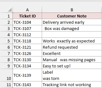
Below I have the ten support tickets from Method #4, including the note with a line break and the one with a nonbreaking space.

I want the word count of each note in column C.

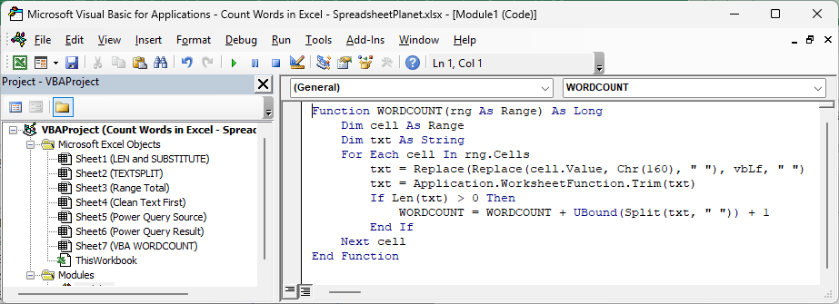
Here is the VBA code:

Function WORDCOUNT(rng As Range) As Long
    Dim cell As Range
    Dim txt As String
    For Each cell In rng.Cells
        txt = Replace(Replace(cell.Value, Chr(160), " "), vbLf, " ")
        txt = Application.WorksheetFunction.Trim(txt)
        If Len(txt) > 0 Then
            WORDCOUNT = WORDCOUNT + UBound(Split(txt, " ")) + 1
        End If
    Next cell
End Function

Function WORDCOUNT(rng As Range) As Long
    Dim cell As Range
    Dim txt As String
    For Each cell In rng.Cells
        txt = Replace(Replace(cell.Value, Chr(160), " "), vbLf, " ")
        txt = Application.WorksheetFunction.Trim(txt)
        If Len(txt) > 0 Then
            WORDCOUNT = WORDCOUNT + UBound(Split(txt, " ")) + 1
        End If
    Next cell
End Function

Here are the steps to add this function to your workbook:

1. Press Alt + F11 to open the VBA Editor
2. Click Insert, then Module
3. Paste the code above into the module window
4. Close the VBA Editor to go back to Excel

Now you can use it in the worksheet. Here is the formula I entered in C2 and copied down to C11:

=WORDCOUNT(B2)

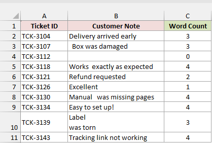
It returns the same counts as Method #4, including 3 for TCK-3139 and 4 for TCK-3143.

The function also takes a whole range. Here is the formula I entered in B13 to get the total for all ten notes:

=WORDCOUNT(B2:B11)

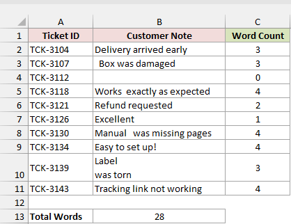
It returns 28.

How does this code work?

The code goes through each cell in the range you give it. For each one, it replaces nonbreaking spaces (Chr(160)) and line breaks (vbLf) with regular spaces.

It then runs Excel’s TRIM function on the text to remove the extra spaces.

If there’s any text left, Split breaks it into words at each space.

UBound returns the position of the last word, counting from 0, so the code adds 1 to get the word count.

The counts for all the cells are added together, which is why the same function works for one cell or a whole range.

Note: Save the file as an Excel Macro-Enabled Workbook (.xlsm) to keep the function. If you save it as a regular .xlsx file, the code is removed.

Additional Notes About Counting Words in Excel

• These methods count groups of characters separated by spaces. Punctuation stays attached to its word, so “up!” is one word, and so is a hyphenated word like follow-up.
• A dash with a space on each side counts as a word of its own, because the formula sees text between two spaces.
• Numbers count as words too. “Order 42 delayed” returns 3.
• If a count looks wrong on text you pasted from somewhere else, check for line breaks and nonbreaking spaces first, and use Method #4.

Frequently Asked Questions

Here are answers to a few common questions about counting words in Excel.

How do I count how many times a specific word appears in Excel?

Use the same idea with the word instead of a space.

Take the length of the text, subtract its length after SUBSTITUTE removes the word, and divide by the word’s length.

I cover this step by step in how to count how many times a word appears in Excel.

What’s the difference between counting words and counting cells with text?

These formulas count the words inside cells. Functions like COUNTA or COUNTIF count how many cells hold something, no matter how many words are in each one.

If that’s what you need, see how to count cells that contain text.

Why does my word count formula return 1 for an empty cell?

The formula adds 1 to the number of spaces, and an empty cell has 0 spaces.

So you get 1 unless the formula checks for empty cells first, like the IF in Method #1 or the (TRIM(B2:B9)<>””) part in Method #3.

Why does my SUMPRODUCT word count formula need Ctrl + Shift + Enter?

It probably has an IF inside it.

In Excel 2019 and older, IF only works on a whole range inside an array formula, which you confirm with Ctrl + Shift + Enter.

The Method #3 formula avoids IF, so pressing Enter is enough.

Conclusion

In this article, I showed you six ways to count words in Excel, from the LEN, TRIM, and SUBSTITUTE formula to Power Query and a custom VBA function.

The Method #1 formula is the one I use most, since it works in every version of Excel.

I hope you found this article helpful.

Other Excel articles you may also like:

• Count Characters in a Cell in Excel
• SUBSTITUTE Function in Excel
• LEN Function in Excel
• COUNTA Function in Excel
• COLUMNS Function in Excel
• Extract Last Word in Excel