
A slicer makes it easy to see what you’ve filtered while you’re looking at it.
But the moment you want that selection in a cell, for a report heading or a chart title, Excel doesn’t offer an option for it.
There’s no SLICER function, and a slicer isn’t a range a formula can point to.
What you can do is read the selection from something the slicer controls, then put the result in a cell.
In this article, I’ll show you four ways to put the slicer selection in a cell: a helper PivotTable with TEXTJOIN, a FILTER formula, CUBE functions, and a VBA macro.
I’ll also show you how to use that cell in a chart title and other formulas.
Method #1: Using a Helper PivotTable and TEXTJOIN
This is the method I’d use for most slicers. It works with any regular PivotTable slicer, doesn’t need macros, and updates the moment you click.
The idea is a second, tiny PivotTable that lists only the items the slicer lets through. A formula then joins that list into one cell.
Below I have a PivotTable that shows plant revenue by store, built from a Table of garden-centre orders.
It has a slicer for the Category field, with Ferns and Orchids selected.
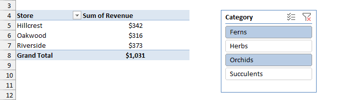
I want cell B1 to show the categories picked in the slicer.
Here are the steps to build the helper PivotTable:
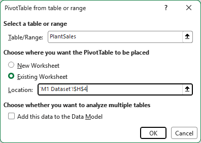
- Select any cell in the source Table, go to the Insert tab, and click PivotTable (pick From Table/Range if you see a drop-down). Choose Existing Worksheet, set the location to cell H4, and click OK.
- In the PivotTable Fields pane, check Category. Don’t add anything to Values. You’ll get a list of the categories with a Grand Total row at the bottom.
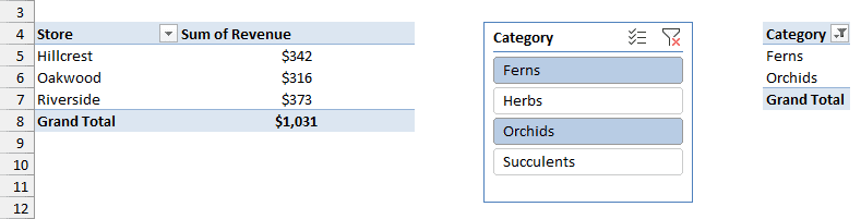
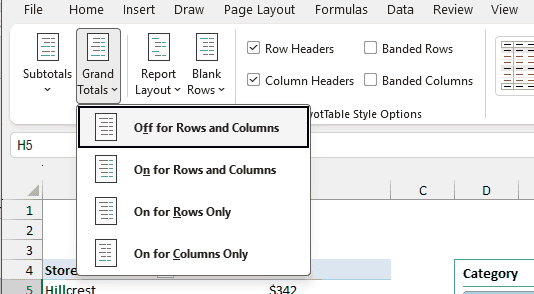
That Grand Total row would end up in your list of selected items, so it has to go.
- With a cell in the helper PivotTable selected, go to the Design tab, click Grand Totals, and choose Off for Rows and Columns.
Right now the slicer only controls the main PivotTable. You need to connect it to the helper too, the same way you’d connect a slicer to multiple PivotTables.
- Right-click the slicer and choose Report Connections. Check the helper PivotTable (mine is named SelectedCategories) and click OK.
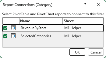
Now the helper list shows only Ferns and Orchids, the same items selected in the slicer.
All that’s left is joining the list into one cell. Here is the formula I entered in B1:
=TEXTJOIN(", ",TRUE,H5:H20)
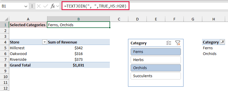
B1 now reads “Ferns, Orchids”. Click a different category in the slicer, and the cell changes with it.
How does this formula work?
TEXTJOIN joins text from a range, putting the first argument (a comma and a space) between each item.
The second argument, TRUE, tells it to skip empty cells.
I pointed it at H5:H20, which is more rows than the helper list will ever need.
The empty cells below the list get ignored, so the range covers every selection size.
I started at H5 so the header in H4 stays out of the result.
Showing “All Categories” Instead of the Full List
There’s one thing that looks odd. When nothing is filtered, the helper lists every category, so B1 shows all four names.
A label like “All Categories” reads better in a report heading. Below, I’ve cleared the slicer and entered this formula in B2:
=IF(COUNTA(H5:H20)=ROWS(UNIQUE(PlantSales[Category])),"All Categories",B1)
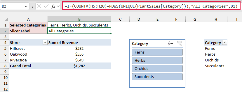
How does this formula work?
COUNTA counts how many items the helper list shows. UNIQUE pulls the distinct categories from the Category column of the source Table (named PlantSales), and ROWS counts them.
When the two numbers match, every category is in, so the formula returns “All Categories”. Otherwise, it returns the list from B1.
Selecting every item by hand gives the same “All Categories” result as clearing the slicer, which is what you’d want.
UNIQUE needs Microsoft 365 or Excel 2021. In Excel 2019, replace ROWS(UNIQUE(PlantSales[Category])) with the number of categories, which is 4 here.
Note: If you only ever pick one item, you can skip TEXTJOIN. Drag Category to the helper PivotTable’s Filters area instead of Rows. Its filter cell then shows the selected item, “(Multiple Items)” or “(All)”.
Method #2: Using SUBTOTAL and FILTER (Table Slicers)
You can also add a slicer to a regular Excel Table, with no PivotTable involved.
In that case, there’s nothing to copy as a helper, but a formula can read the selection straight from the Table.
When a Table slicer filters, it hides the rows that don’t match. This method lists the categories in the rows that are still visible.
Below I have the same orders in an Excel Table named PlantOrders, with a Category slicer. Ferns and Orchids are selected, so the Table shows only those six orders.
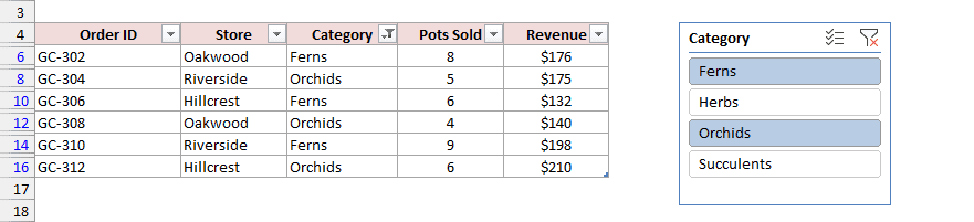
Here is the formula I entered in B1:
=TEXTJOIN(", ",TRUE,SORT(UNIQUE(FILTER(PlantOrders[Category],MAP(PlantOrders[Category],LAMBDA(c,SUBTOTAL(103,c)))))))
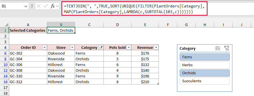
It returns “Ferns, Orchids”, matching the slicer.
How does this formula work?
The trick is SUBTOTAL with 103 as its first argument. That counts non-empty cells, but it ignores any row a filter has hidden.
MAP runs SUBTOTAL(103,c) on each Category cell one at a time. A visible cell returns 1 and a hidden cell returns 0.
FILTER keeps the categories where MAP returned 1.
UNIQUE removes the repeats, SORT puts them in A to Z order (the order the slicer shows them), and TEXTJOIN joins them with a comma.
This formula needs MAP and LAMBDA, so it works in Microsoft 365 and Excel 2024.
You can handle the “nothing filtered” case here too. In B2, I entered this formula, and below you can see it with the slicer cleared:
=IF(SUBTOTAL(103,PlantOrders[Category])=ROWS(PlantOrders),"All Categories",B1)
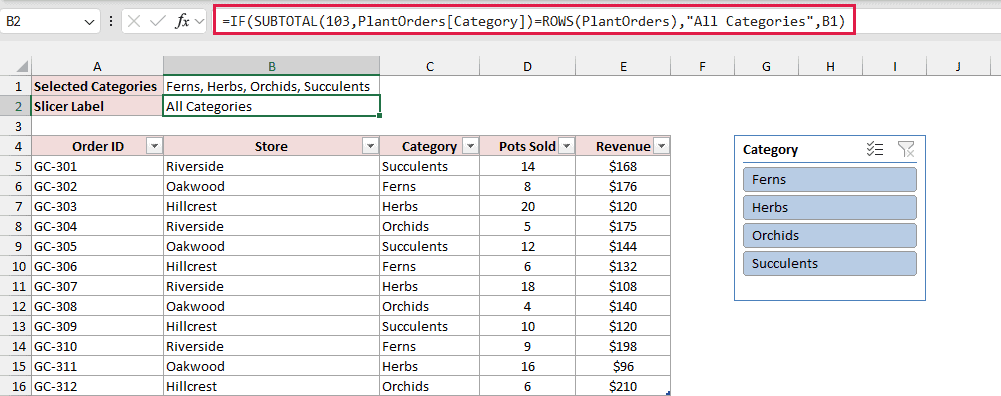
SUBTOTAL(103) counts the visible rows, and ROWS counts every row in the Table. When they match, nothing is hidden, so the formula returns “All Categories”.
Note: Keep these formula cells above or beside the Table, never in rows next to it. When the slicer hides a row, anything else in that row gets hidden too.
Method #3: Using CUBE Functions (Data Model Slicers)
If your PivotTable is built on the Data Model, you don’t need a helper at all. Excel’s CUBE functions can read a Data Model slicer directly by its name.
These functions only work with Data Model slicers. On a regular PivotTable slicer, they return #N/A.
Below I have a PivotTable of revenue by store, built from the same plant sales data, with a Category slicer. Ferns and Orchids are selected.
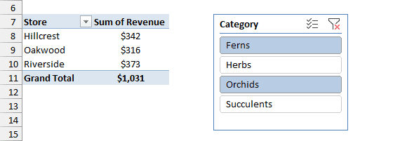
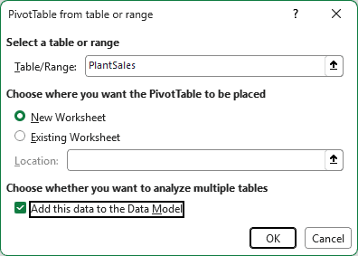
The difference is in how I created it. In the PivotTable from table or range dialog box, I checked Add this data to the Data Model before clicking OK.
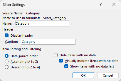
The CUBE formulas refer to the slicer by name, so you’ll need that name first.
Right-click the slicer and choose Slicer Settings. The name is next to Name to use in formulas. Mine is Slicer_Category.
Let me start with the first selected item. Here is the formula I entered in B1:
=CUBERANKEDMEMBER("ThisWorkbookDataModel",Slicer_Category,1)
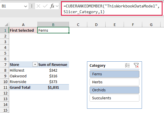
It returns Ferns.
CUBERANKEDMEMBER returns the item at a given position in a set.
“ThisWorkbookDataModel” is the name Excel gives the workbook’s Data Model. Slicer_Category is the set of items selected in the slicer, and 1 asks for the first one.
To get all the selected items, you first need to know how many there are. Here is the formula I entered in B2:
=CUBESETCOUNT(Slicer_Category)
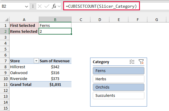
It returns 2, because two categories are selected.
Now you can ask CUBERANKEDMEMBER for items 1 and 2 in one go. In H2, I entered this formula, and it spills the selected items down the column:
=CUBERANKEDMEMBER("ThisWorkbookDataModel",Slicer_Category,SEQUENCE(CUBESETCOUNT(Slicer_Category)))
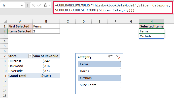
SEQUENCE(CUBESETCOUNT(Slicer_Category)) returns the numbers 1 and 2. CUBERANKEDMEMBER returns one item for each number, so you get a spilled list that grows and shrinks with the slicer.
If you want all of them in a single cell instead, wrap the same formula in TEXTJOIN. Here is the formula I entered in B3:
=TEXTJOIN(", ",TRUE,CUBERANKEDMEMBER("ThisWorkbookDataModel",Slicer_Category,SEQUENCE(CUBESETCOUNT(Slicer_Category))))
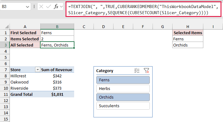
It returns “Ferns, Orchids”.
When nothing is filtered, the CUBE functions behave differently from the other methods.
CUBESETCOUNT returns 1 and CUBERANKEDMEMBER returns “All”, so B3 reads “All”. That’s usually a fine label as it is.
The slicer name also works inside CUBEVALUE, which returns a total for whatever the slicer selects. Here is the formula I entered in B4:
=CUBEVALUE("ThisWorkbookDataModel","[Measures].[Sum of Revenue]",Slicer_Category)
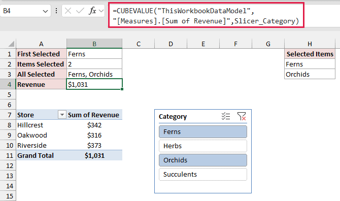
It returns $1,031, the revenue for Ferns and Orchids, matching the PivotTable’s grand total. [Measures].[Sum of Revenue] is the measure Excel created when I added Revenue to the Values area.
Note: CUBE formulas show #GETTING_DATA for a moment after a slicer click while Excel queries the Data Model. That’s normal. The result appears a second later.
Method #4: Using a VBA Event Macro
A macro is the way to go if you’re on an older version of Excel without TEXTJOIN, or you’d rather not keep a helper PivotTable around.
The macro runs every time the PivotTable updates, which happens whenever you click the slicer. It reads the slicer’s selected items and writes them into a cell.
Below I have a PivotTable that shows revenue by category, with a Store slicer. I want B1 to show the stores selected in the slicer.
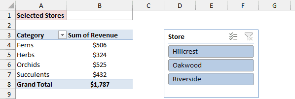
Here is the VBA code:
Private Sub Worksheet_PivotTableUpdate(ByVal Target As PivotTable)
    Dim sc As SlicerCache
    Dim si As SlicerItem
    Dim txt As String

    Set sc = ThisWorkbook.SlicerCaches("Slicer_Store")

    If sc.FilterCleared Then
        txt = "All Stores"
    Else
        For Each si In sc.SlicerItems
            If si.Selected Then txt = txt & ", " & si.Name
        Next si
        txt = Mid(txt, 3)
    End If

    Me.Range("B1").Value = txt
End SubHere are the steps to use this macro:
- Right-click the tab of the sheet that has the PivotTable and choose View Code. This opens the code window for that sheet.
- Paste the code above into the code window.
- Change Slicer_Store to your slicer’s name (right-click the slicer and choose Slicer Settings to find it), and B1 to the cell you want.
- Close the VBA Editor and click a few items in the slicer.
Below, I’ve selected Oakwood and Riverside, and B1 shows “Oakwood, Riverside”.
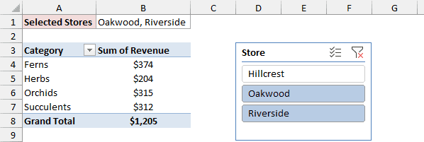
Worksheet_PivotTableUpdate is an event, so Excel runs it on its own each time a PivotTable on that sheet changes.
The code goes through every item in the slicer and adds the selected ones to a text string, with a comma before each.
Mid(txt, 3) then removes the extra comma and space at the front.
If the slicer is cleared, or every store is selected, FilterCleared is True and the macro writes “All Stores” instead.
Note: Save the file as an Excel Macro-Enabled Workbook (.xlsm), or the code is removed when you save. The code must go in the sheet’s own code window, not a regular module, or the event never runs.
How to Use the Slicer Selection in a Formula
Once the selection is in a cell, you can use it anywhere a formula can reach. Here are three ways to use it.
All three use the helper PivotTable from Method #1. Below, the helper list is in H6 onwards, and B1 has the selection with the “All Categories” check built in:
=IF(COUNTA(H6:H20)=ROWS(UNIQUE(PlantSales[Category])),"All Categories",TEXTJOIN(", ",TRUE,H6:H20))
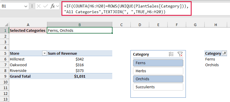
It’s the TEXTJOIN formula and the “All Categories” check from Method #1 combined into one cell.
Creating a Dynamic Chart Title
A chart title can’t hold a formula, but you can make it a dynamic chart title that points to a cell. So I first build the title text in B2:
="Revenue by Store: "&B1
Then, to link the chart title to it:
- Click the chart title to select it.
- Click in the formula bar, type an equal sign (=), then click cell B2 and press Enter.
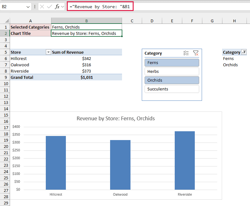
The chart title now reads “Revenue by Store: Ferns, Orchids”, and it changes each time you click the slicer.
Building a Label With GETPIVOTDATA
You can also combine the selection with a number from the PivotTable. Here is the formula I entered in B3:
="Revenue for "&B1&": "&TEXT(GETPIVOTDATA("Revenue",$A$5),"$#,##0")
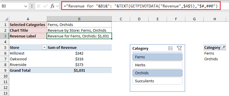
It returns “Revenue for Ferns, Orchids: $1,031”.
GETPIVOTDATA(“Revenue”,$A$5) returns the grand total of the Revenue field from the PivotTable that starts in A5.
Since the slicer filters that PivotTable, the total follows the selection. TEXT formats it as a dollar amount.
Pulling the Matching Rows With FILTER
The helper list also works as criteria. This formula returns every order in the selected categories. I entered it in J6, under a row of headers I typed in J5:N5:
=FILTER(PlantSales,ISNUMBER(XMATCH(PlantSales[Category],H6:H20)))
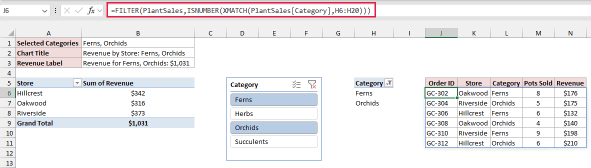
It spills the six Ferns and Orchids orders.
XMATCH looks up each order’s category in the helper list.
It returns a position for a match and #N/A otherwise. ISNUMBER turns that into TRUE or FALSE, and FILTER keeps the TRUE rows.
Which Method Should You Use?
Here’s a quick way to choose, based on the kind of slicer you have.
| Your slicer | Method | Excel version | When nothing is filtered |
|---|---|---|---|
| Regular PivotTable slicer | #1 Helper PivotTable and TEXTJOIN | Excel 2019 or later (the check needs Microsoft 365 or Excel 2021) | Every item (or “All Categories” with the check) |
| Excel Table slicer | #2 SUBTOTAL and FILTER | Microsoft 365 or Excel 2024 | Every item (or “All Categories” with the check) |
| Data Model PivotTable slicer | #3 CUBE functions | Excel 2013 or later (SEQUENCE needs Microsoft 365 or Excel 2021) | “All” |
| Any PivotTable slicer | #4 VBA event macro | Excel 2010 or later | “All Stores” |
Additional Notes About Showing Slicer Selection in Excel
- Keep the cells below the helper PivotTable empty. The list gets longer when you select more items, so it needs room to grow.
- The helper PivotTable can live on another sheet or in hidden columns. The slicer still controls it, and your formulas still read it.
- The VBA macro doesn’t run in Excel for the web. There, the cell keeps its last value until you open the file in the desktop app.
- Slicers update the cell instantly, but if you add orders to the source data, refresh the PivotTables with Data > Refresh All so they (and the helper list) pick them up.
Frequently Asked Questions
Here are a few more questions about slicer selections.
Can I change a slicer based on a cell value?
A formula can read a slicer but can’t change it.
You’d need a macro that sets each slicer item’s Selected property based on the cell, run from a Worksheet_Change event.
How do I show only the first selected item?
With the helper PivotTable from Method #1, use =INDEX(H5:H20,1). With a Data Model slicer, use CUBERANKEDMEMBER with 1 as the last argument, as in Method #3.
Why does “(blank)” appear in my list?
Your source data has empty cells in the slicer’s field, and the PivotTable lists them as “(blank)”.
Fill in the empty cells, or leave the item out with =TEXTJOIN(“, “,TRUE,FILTER(H5:H20,H5:H20<>”(blank)”,””)).
This needs FILTER, so it works in Microsoft 365 and Excel 2021 or later.
I don’t have TEXTJOIN. What can I use?
TEXTJOIN arrived in Excel 2019. In Excel 2016 or earlier, use the VBA macro from Method #4.
For a single selection, the Filters area trick in the Method #1 note also works in any version.
Conclusion
In this article, I showed you four ways to put a slicer’s selection in a cell.
I also showed you how to use that cell in a chart title, a label, and a FILTER formula.
For most PivotTable slicers, the helper PivotTable with TEXTJOIN is the one I’d start with.
I hope you found this article helpful.
Other Excel articles you may also like:
