How to Convert Date to Fiscal Year in Excel (4 Easy Ways)

A fiscal year is the 12-month period a company or government uses for its accounts, and it often doesn’t start in January.

If your fiscal year runs from July to June, an invoice from August 2026 belongs to fiscal year 2027. Excel’s YEAR function would still return 2026.

So you need a formula that checks the month of each date and moves the later months into the next year.

There’s one more wrinkle. Most organizations name a fiscal year after the year it ends in, so July 2025 to June 2026 is FY2026.

Some use the year it starts in instead.

In this article, I’ll show you four ways to convert a date to a fiscal year, using YEAR and MONTH, the EDATE function, a custom LAMBDA function, and Power Query.

I’ll also show you how to display the result as FY2026 or 2025-26, and what to change if your fiscal year is named by its start year.

Table of Contents

Method #1: Using the YEAR and MONTH Functions

This is the method I recommend for most people. It’s one short formula, and you can switch to a different fiscal year start by changing a single cell.

Below I have a dataset on the YEAR and MONTH sheet. It’s a purchase order log, with each order date in column B.

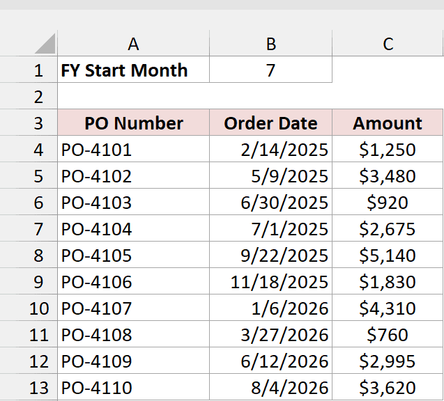
Purchase order log with PO number, order date, and amount, and the fiscal year start month 7 in cell B1

The fiscal year starts in July, so cell B1 holds 7, the number for July. I want the fiscal year of each order in column D.

Here is the formula:

=YEAR(B4:B13)+(MONTH(B4:B13)>=$B$1)

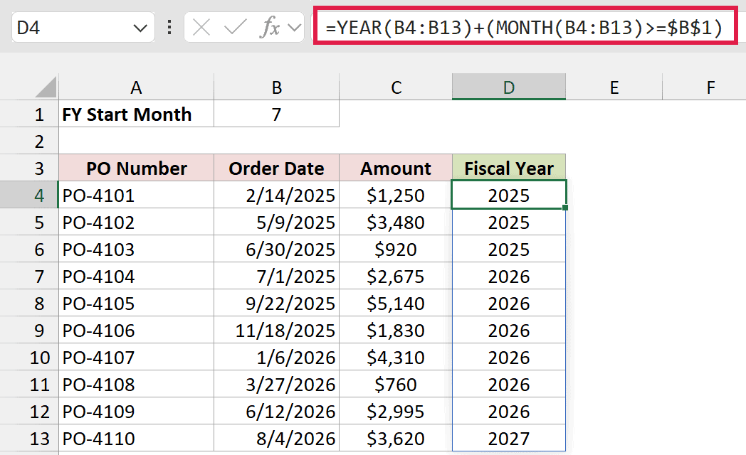
YEAR and MONTH formula in D4 returning the fiscal year of each order

Enter it in D4, and it spills down the column automatically. PO-4103 on 6/30/2025 stays in fiscal year 2025, while PO-4104 on 7/1/2025 moves to fiscal year 2026.

How does this formula work?

The YEAR function returns the calendar year of each date, like 2025 for 7/1/2025.

The MONTH function returns the month number, from 1 to 12. The comparison MONTH(B4:B13)>=$B$1 checks whether that month is July or later.

That check returns TRUE or FALSE. When you add it to a number, Excel treats TRUE as 1 and FALSE as 0.

So dates from July to December get 1 added to their year, and dates from January to June keep their calendar year.

If your fiscal year starts in April, change B1 to 4. For an October start, like the US federal government, change it to 10.

Note: Spilling formulas need Excel 365 or Excel 2021 and later. In older versions, enter =YEAR(B4)+(MONTH(B4)>=$B$1) in D4 and copy it down the column.

Method #2: Using the EDATE Function

Here’s another way to think about it. Instead of checking the month, you shift every date forward so the fiscal year lines up with the calendar year.

A bonus of this method is that the same shifted date also gives you the fiscal month.

Below I have the same purchase order log on the EDATE sheet, with the order dates in column B and the start month (7) in cell B1.

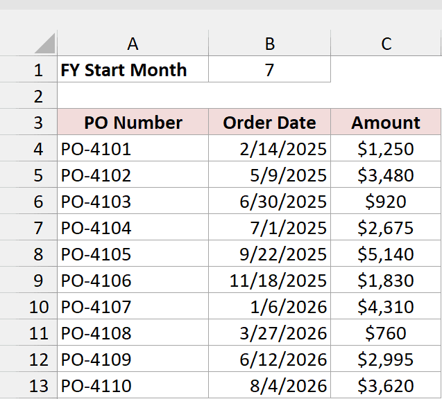
I want the fiscal year in column D and the fiscal month in column E.

Here is the formula for the fiscal year:

=YEAR(EDATE(B4,13-$B$1))

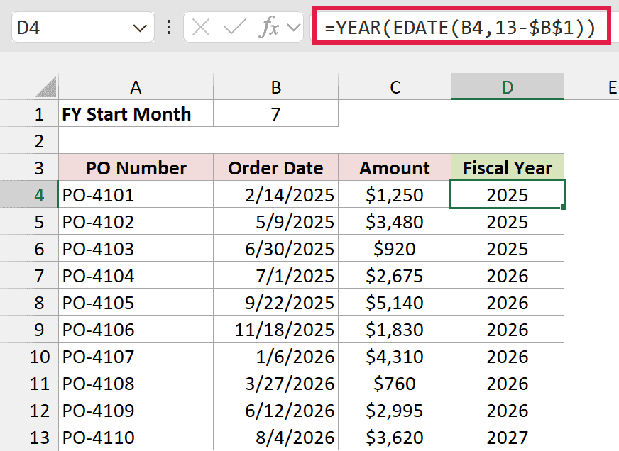
EDATE formula in D4 returning the fiscal year, copied down column D

Enter it in D4, then double-click the fill handle to copy it down. EDATE doesn’t accept a whole range, so this formula has to go row by row.

The results match Method #1. PO-4110 on 8/4/2026 is in fiscal year 2027.

How does this formula work?

The EDATE function returns the date a given number of months before or after a date.

With 7 in B1, 13-$B$1 is 6, so EDATE moves every date 6 months forward. July 1, 2025 becomes January 1, 2026.

Because July always lands in January of the next year, YEAR returns the right fiscal year for every date.

June 30, 2025 moves to December 30, 2025, so it stays in 2025.

Now for the fiscal month. Enter this formula in E4 and copy it down:

=MONTH(EDATE(B4,13-$B$1))

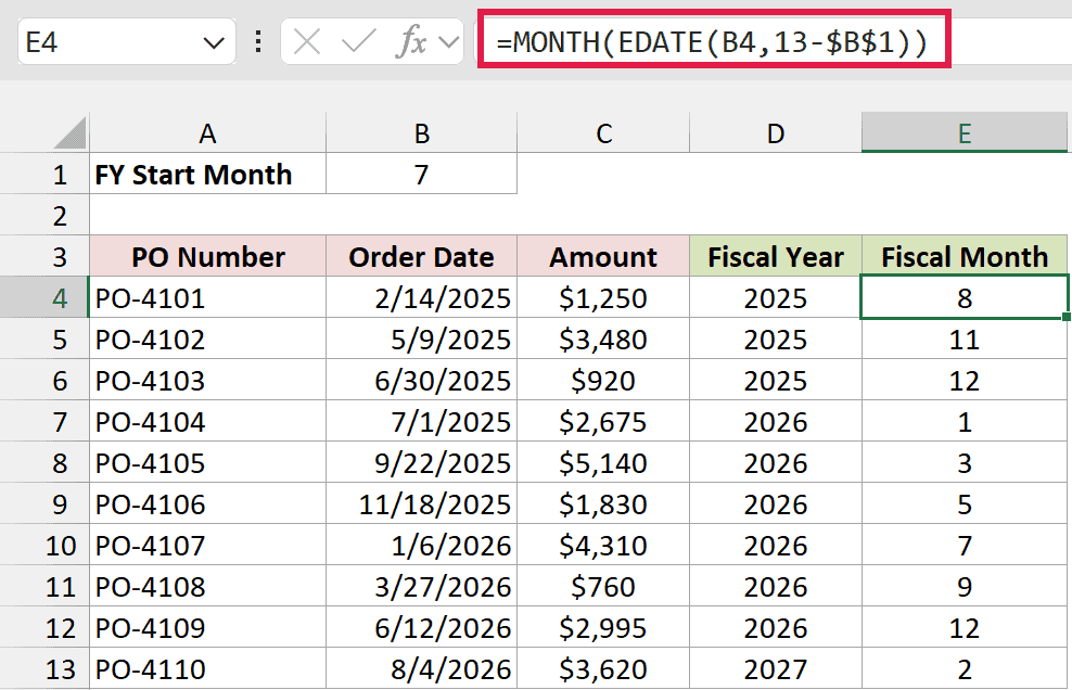
MONTH and EDATE formula in E4 returning the fiscal month, with July as month 1

Since July becomes January after the shift, MONTH returns 1 for July, 2 for August, and so on. June, the last month of the fiscal year, returns 12.

PO-4101 on 2/14/2025 is in fiscal month 8, because February is the eighth month of a July-to-June year.

Method #3: Using a Custom LAMBDA Function

If you calculate fiscal years in a lot of places, you can turn the formula into your own function. Once it’s set up, you type =FISCALYEAR() like any built-in function.

This uses the LAMBDA function, which is available in Excel 365 and Excel 2024.

Below I have the purchase order log on the LAMBDA sheet, with the order dates in column B and the start month (7) in cell B1.

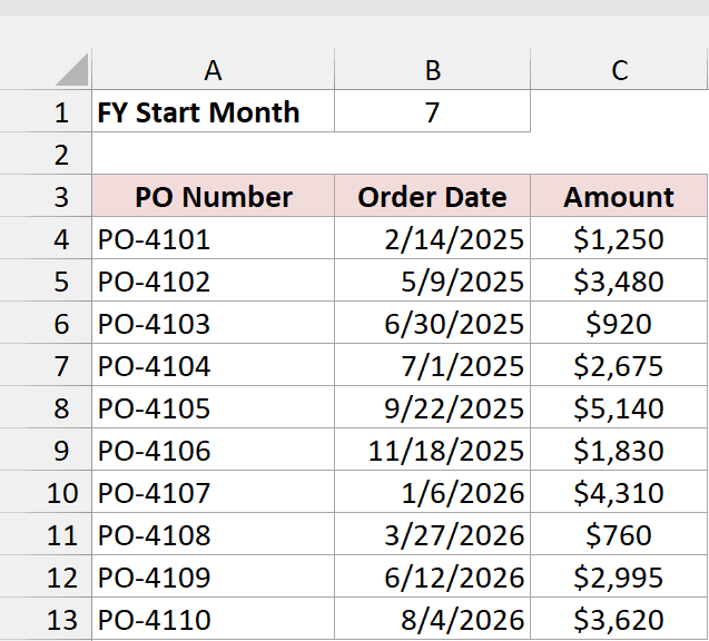
Here are the steps to create the FISCALYEAR function:

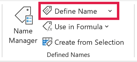
Go to the Formulas tab and click Define Name.

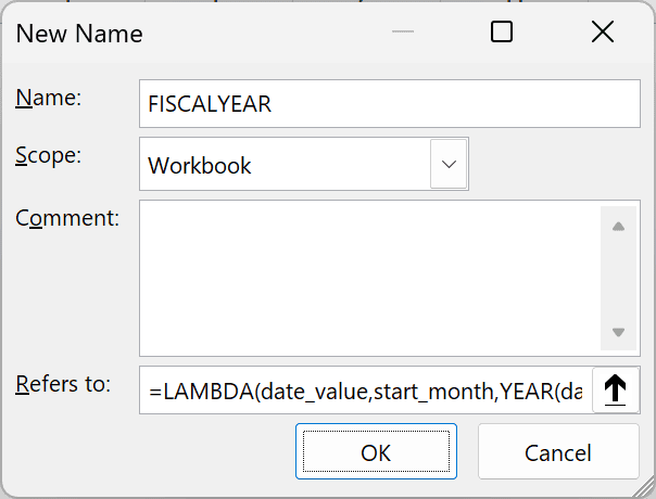
In the New Name dialog box, type FISCALYEAR in the Name field. Paste the formula below into the Refers to field, then click OK.

=LAMBDA(date_value,start_month,YEAR(date_value)+(MONTH(date_value)>=start_month))

New Name dialog with FISCALYEAR as the name and the LAMBDA formula in Refers to

Now you can use it on the sheet. Enter this formula in D4:

=FISCALYEAR(B4:B13,$B$1)

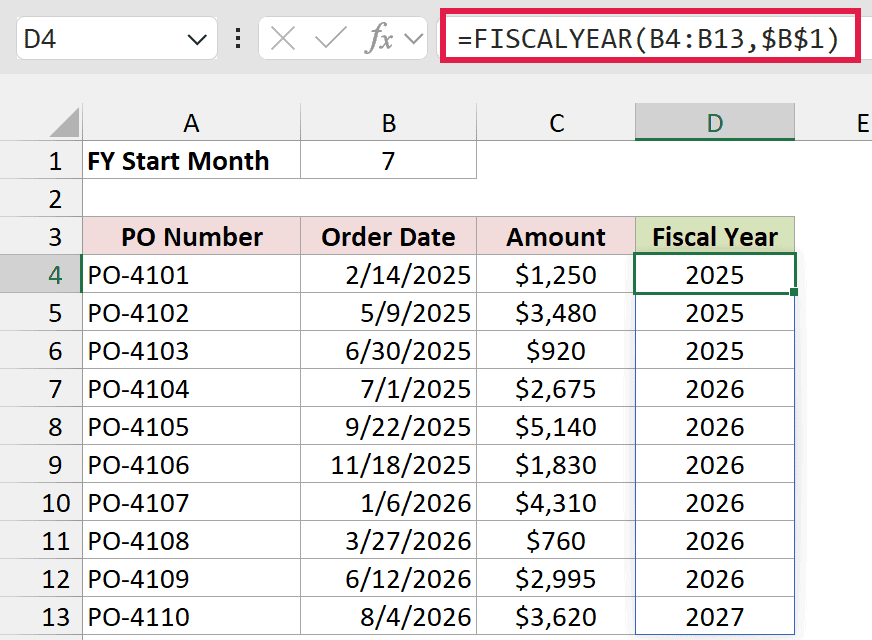
Custom FISCALYEAR function in D4 returning the fiscal year of each order

It spills down the column and returns the same fiscal years as Method #1.

How does this work?

The LAMBDA function lets you build a function from a formula. The names before the last argument, date_value and start_month, are the inputs your function takes.

The last argument is the calculation. It’s the Method #1 formula, with the cell references swapped for those two inputs.

When you enter =FISCALYEAR(B4:B13,$B$1), Excel passes the dates in as date_value and 7 as start_month.

Note: FISCALYEAR is saved in this workbook only. To use it in another workbook, define the name there too, or copy a sheet that uses it into that workbook.

Method #4: Using Power Query

If you get your data as an export you refresh often, Power Query can add the fiscal year column for you each time.

Below I have the purchase order log on the Power Query Source sheet. It needs to be an Excel Table for Power Query to pick it up.

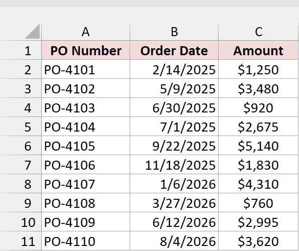
Purchase order log with PO number, order date, and amount in A1:C11

Here are the steps to add a fiscal year column with Power Query:

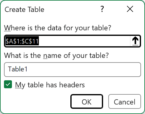
If your data isn’t a table yet, select any cell in it and press Ctrl + T (Cmd + T on a Mac). Make sure My table has headers is checked, then click OK.

Create Table dialog with the range A1:C11 and My table has headers checked

Go to the Data tab and click From Table/Range. The Power Query Editor opens with your table.

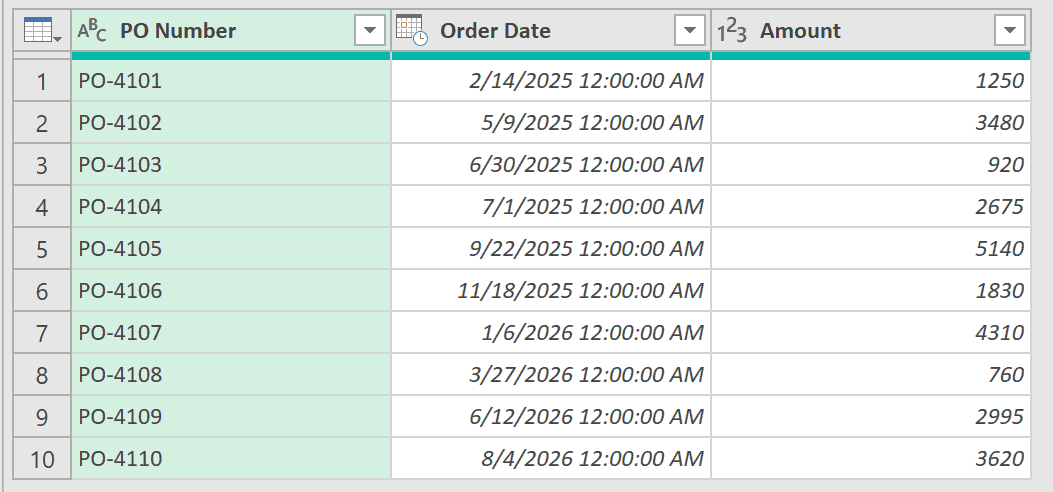
Purchase order table opened in the Power Query Editor, with a date-and-time icon on Order Date

If the Order Date header shows a date-and-time icon, click that icon and choose Date. When Power Query asks, click Replace current.

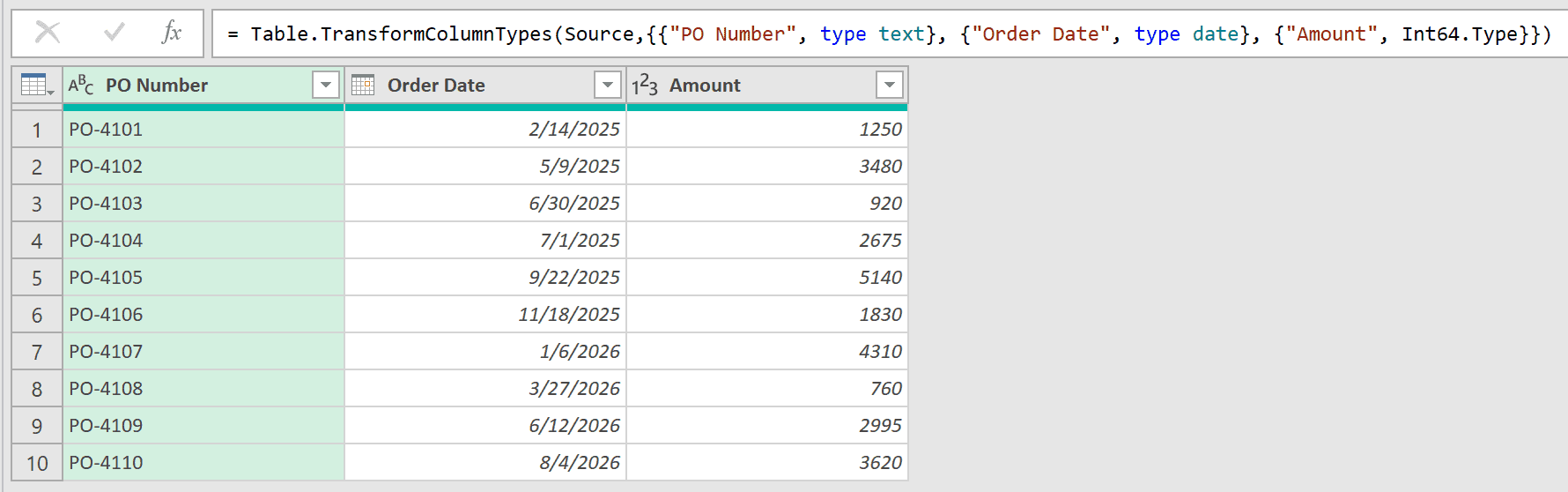
Changed Type step with the Order Date column set to the Date type

Without this step, the loaded table shows a time of 12:00:00 AM next to every order date.

Go to the Add Column tab and click Custom Column.

Custom Column button on the Add Column tab of the Power Query Editor

Type Fiscal Year as the New column name. Enter the formula below in the Custom column formula box, then click OK.

if Date.Month([Order Date]) >= 7 then Date.Year([Order Date]) + 1 else Date.Year([Order Date])

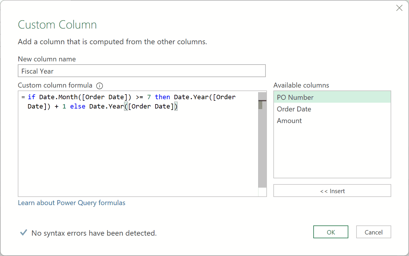
Custom Column dialog with Fiscal Year as the column name and the if formula

This is the same logic as Method #1. Date.Month and Date.Year are Power Query’s versions of MONTH and YEAR.

Orders from July onward get 1 added to their year. Change the 7 if your fiscal year starts in a different month.

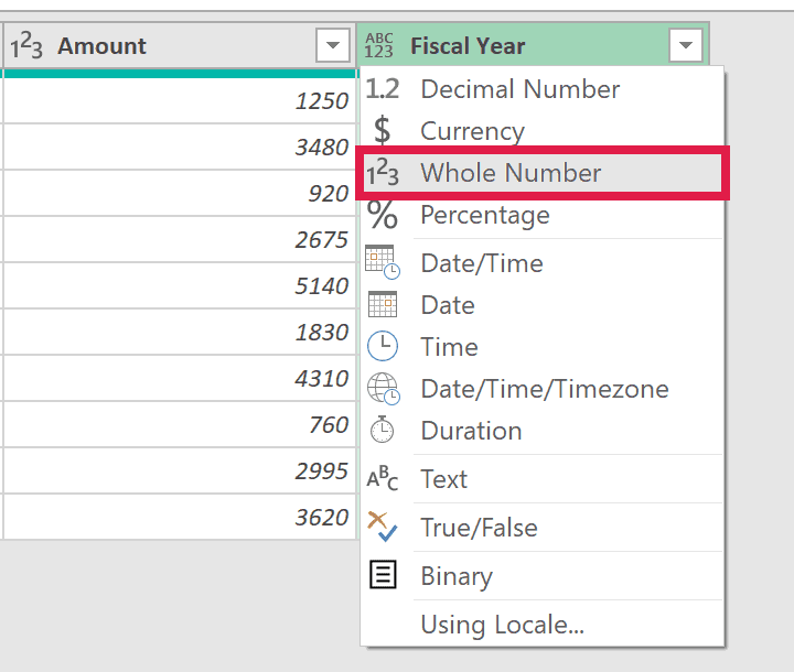
Click the ABC123 icon in the Fiscal Year header and choose Whole Number.

Data type menu on the Fiscal Year column with Whole Number highlighted

On the Home tab, click Close & Load.

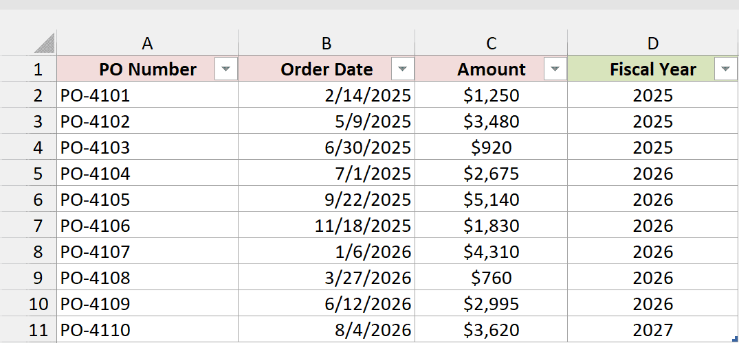
Power Query result loaded to a new sheet with the Fiscal Year column

Power Query loads the result as a new table on a new sheet, with the fiscal year of each order in the Fiscal Year column.

Note: The loaded table doesn’t update by itself. When you add or change orders in the source table, go to the Data tab and click Refresh All.

How to Show the Fiscal Year as FY2026 or 2025-26

A plain number like 2026 works fine for sorting and lookups. In reports, though, you’ll often see fiscal years written as FY2026, or as a range like 2025-26.

Below I have the purchase order log on the FY Labels sheet. Column D already has the fiscal year from the Method #1 formula.

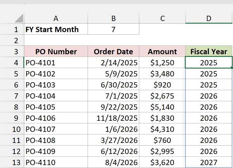
Purchase order log with the fiscal year of each order in column D

To add the FY prefix, enter this formula in E4:

="FY"&D4:D13

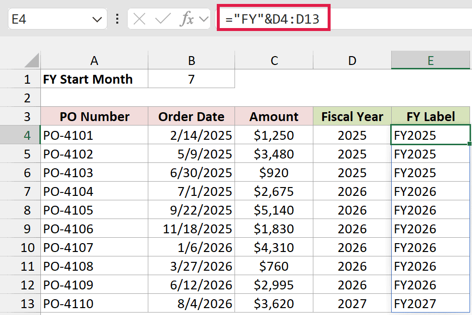
Formula in E4 adding the FY prefix to each fiscal year

The & operator joins the text FY to each year, so 2026 becomes FY2026.

For a range label like 2025-26, enter this formula in F4:

=(D4:D13-1)&"-"&RIGHT(D4:D13,2)

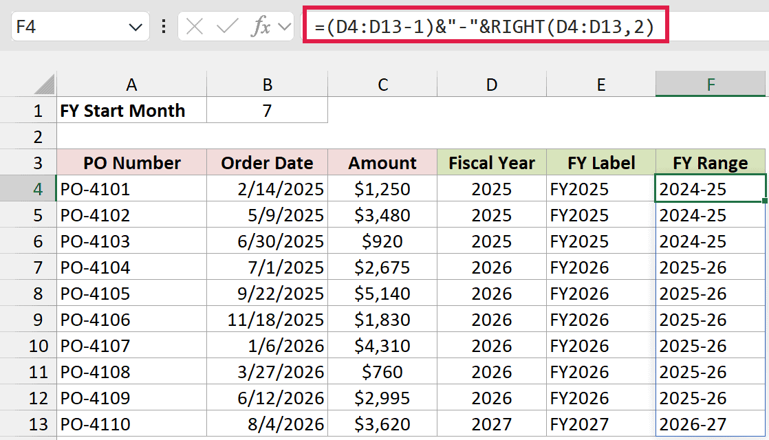
Formula in F4 returning fiscal year range labels like 2025-26

D4:D13-1 returns the year the fiscal year starts in. The RIGHT function takes the last two digits of the year it ends in, so fiscal year 2026 becomes 2025-26.

Both labels are text. Keep the number column for any math, and use the labels for display.

How to Get a Fiscal Year Named by Its Start Year

Some organizations name a fiscal year after the year it starts in. With a July start, July 2025 to June 2026 is then fiscal year 2025, not 2026.

Below I have the purchase order log on the Start-Year Naming sheet, with the order dates in column B and the start month (7) in cell B1.

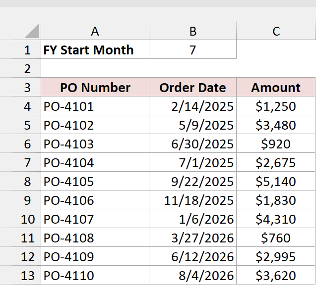
Here is the formula:

=YEAR(B4:B13)-(MONTH(B4:B13)<$B$1)

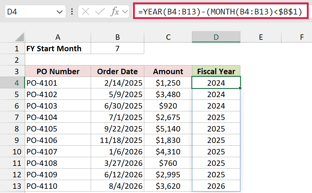
Formula in D4 returning the fiscal year named by the year it starts in

This time, dates before July get 1 subtracted from their year. PO-4103 on 6/30/2025 is in fiscal year 2024, and PO-4104 on 7/1/2025 starts fiscal year 2025.

If you’re not sure which naming your organization uses, check a recent report. If July 2025 to June 2026 is called FY2026, use Method #1.

Additional Notes About Converting Dates to Fiscal Years in Excel

Keep the start month in one cell. Methods #1 to #3 read it from B1, so you can switch from July to April by changing a single number.
Text that looks like a date returns #VALUE! Every method needs real Excel dates. If your dates came in as text, convert text to dates first.
The formulas update on their own; Power Query doesn’t. Change an order date and Methods #1 to #3 recalculate right away. Method #4 needs a refresh.

Frequently Asked Questions

Here are answers to a few questions people often ask about fiscal years in Excel.

Is a financial year the same as a fiscal year?

Yes. Financial year is the term used in the UK, India, and Australia. India’s runs from April to March and is usually written as 2025-26.

The formulas work the same way. Set the start month to 4 for April, or 7 for July.

What if my fiscal year starts in January?

Then your fiscal year is the same as the calendar year, and =YEAR(B4) is all you need.

Don’t put 1 in the start month cell for Methods #1 to #3. They would add 1 to every year.

How do I get the fiscal quarter from a date?

Start with the fiscal month from Method #2, then divide it by 3 and round up with the ROUNDUP function. Fiscal month 8 is in fiscal quarter 3.

I cover more ways to do this in how to convert date to quarter in Excel.

Why does my fiscal year show as 7/18/1905 instead of 2026?

The cell has a date format, so Excel shows 2026 as the date with that serial number.

Select the cells, go to the Home tab, and pick General from the Number Format drop-down.

Can a Pivot Table group dates by fiscal year?

Not with its Group option, which only groups dates by calendar periods like months, quarters, and years.

Add a Fiscal Year column to your source data with one of the methods above, refresh the Pivot Table, and drag Fiscal Year to the Rows area.

Conclusion

In this article, I showed you four ways to convert a date to a fiscal year in Excel, using YEAR and MONTH, EDATE, a custom LAMBDA function, and Power Query.

I also covered FY labels and fiscal years named by their start year. For most people, the YEAR and MONTH formula is the one to reach for.

I hope you found this article helpful.

Other Excel articles you may also like: