
If you need to repeat rows in Excel, there’s no Repeat Rows button to do it for you.
You might want each row repeated, the whole list repeated, or a different number of copies for each row, such as one per shelf label you plan to print.
I’ll show you how to use copy and paste, CHOOSEROWS with SEQUENCE, Power Query, and a short VBA macro to repeat rows in Excel.
Method #1: Using Copy and Paste
For a quick copy of the whole list, you can paste into a larger selection. Excel repeats the copied cells when that selection is an exact multiple of the source.
Below I have grocery SKUs and products in A2:B9 on the Copy and Paste sheet, and I want the whole list three times in columns D:E.
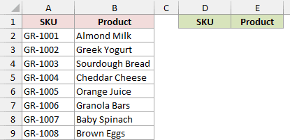
The SKU and Product headers are already typed in D1:E1. Here are the steps to repeat the list:
- Select A2:B9 and press Ctrl + C.
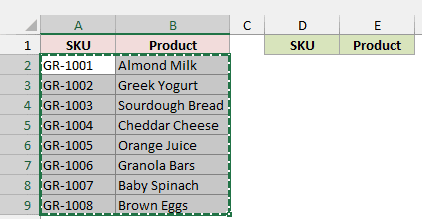
- Select D2:E25. The eight source rows multiplied by 3 need 24 rows. You can type D2:E25 in the Name Box and press Enter to select it.
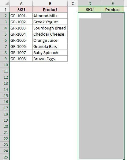
- Press Ctrl + V.
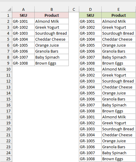
The list is pasted three times, one copy after the other.
The destination must be an exact multiple of the copied range. Select 19 rows for this eight-row list, for example, and Excel pastes the list just once.
These are static values. If the original list changes, paste it again to update the copies.
Note: To repeat a single row, select that row plus the rows below it where the copies should go, then press Ctrl + D. Excel fills the top row down into every selected row.
Method #2: Using CHOOSEROWS and ROUNDUP (Each Row)
If you want each row’s copies grouped together, a formula can do the repeating for you. I recommend this method for most readers.
The CHOOSEROWS function returns rows you specify. Here, I’ll use SEQUENCE and ROUNDUP to request row 1 three times, then row 2 three times, and so on.
Below I have grocery SKUs and products in A2:B9 on the Repeat Each Row sheet, and I want each row repeated three times.
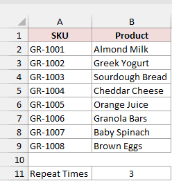
The Repeat Times label is in A11, with 3 in B11. Enter this formula in D2:
=CHOOSEROWS(A2:B9,ROUNDUP(SEQUENCE(ROWS(A2:B9)*B11)/B11,0))
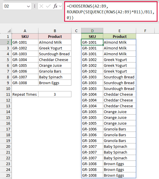
The formula spills 24 rows down columns D:E automatically. Almond Milk appears three times, followed by Greek Yogurt three times, and so on.
How does this formula work?
ROWS(A2:B9) returns 8. Multiplying that by B11 gives 24, the number of output rows we need.
SEQUENCE(24) returns the numbers 1 to 24. Dividing them by 3 gives 0.33, 0.67, 1, 1.33, 1.67, 2, and so on.
ROUNDUP(...,0) rounds those numbers up to whole numbers. The result is 1,1,1,2,2,2, continuing through 8,8,8.
CHOOSEROWS returns those rows from A2:B9. Repeated row numbers produce repeated rows, so changing B11 resizes the result.
CHOOSEROWS needs Microsoft 365 or Excel 2024 on Windows or Mac. Older versions return a #NAME? error.
Method #3: Using CHOOSEROWS and MOD (Whole List)
If you prefer the entire list repeated before it starts again, you can change how the formula generates its row numbers.
Below I have grocery SKUs and products in A2:B9 on the Repeat Whole List sheet, and I want three complete copies of the list.
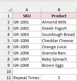
A11 contains Repeat Times, and B11 contains 3. Enter this formula in D2:
=CHOOSEROWS(A2:B9,MOD(SEQUENCE(ROWS(A2:B9)*B11,,0),ROWS(A2:B9))+1)
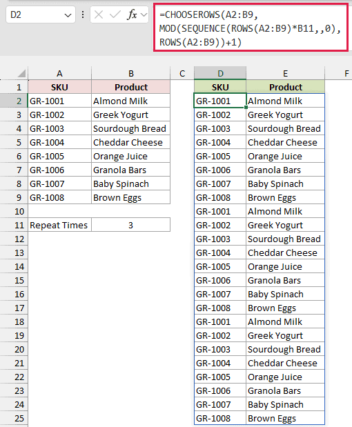
The result spills down to row 25. It runs from Almond Milk to Brown Eggs, then starts over two more times.
How does this formula work?
As before, ROWS(A2:B9)*B11 calculates 24 output rows. This time, SEQUENCE starts its numbers at 0.
Its syntax is SEQUENCE(rows,[columns],[start],[step]). So SEQUENCE(24,,0) returns 24 numbers, from 0 to 23.
The empty second argument keeps the result in one column. The 0 in the third argument sets the starting number.
MOD returns the remainder after division. MOD(...,8) produces 0 to 7 three times, and adding 1 turns that into row numbers 1 to 8 repeating.
CHOOSEROWS returns those rows from A2:B9. ROUNDUP in Method #2 groups the row numbers, while MOD cycles through them.
Method #4: Using CHOOSEROWS and TOCOL (Different Counts)
When each product needs a different number of copies, you can use a count beside each row.
Below I have grocery SKUs, products, and Labels counts in A2:C9 on the Different Counts sheet. I want one output row per label.
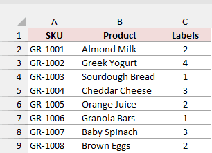
Almond Milk needs 2 labels, Greek Yogurt 4, Sourdough Bread 1, and Cheddar Cheese 3.
Orange Juice needs 2, Granola Bars 1, Baby Spinach 3, and Brown Eggs 2. Enter this formula in E2:
=CHOOSEROWS(A2:B9,TOCOL(IF(SEQUENCE(,MAX(C2:C9))<=C2:C9,SEQUENCE(ROWS(C2:C9)),NA()),2))
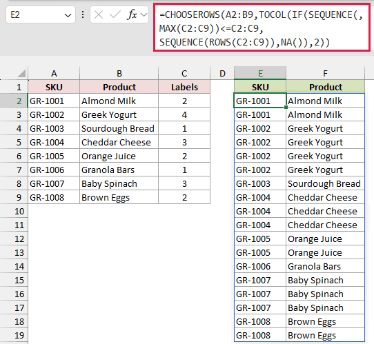
The formula spills 18 rows, the total of the Labels counts. Almond Milk appears twice, Greek Yogurt four times, and the remaining products follow their own counts.
How does this formula work?
MAX(C2:C9) returns 4, the largest count. SEQUENCE(,4) returns 1,2,3,4 across one row.
Comparing those numbers with C2:C9 creates an eight-row by four-column TRUE/FALSE grid. A product needing 2 labels has TRUE in its first two columns.
SEQUENCE(ROWS(C2:C9)) returns row positions 1 to 8. IF returns that position for TRUE and #N/A for FALSE.
TOCOL turns the grid into one column. Its syntax is TOCOL(array,[ignore],[scan_by_column]), and it reads row by row by default.
The second argument, 2, drops errors. That leaves 1,1,2,2,2,2,3, and so on, which CHOOSEROWS uses to return the matching products.
A count of 0, or a blank count cell, drops that product from the result. TOCOL also needs Microsoft 365 or Excel 2024.
Method #5: Using Power Query
For data that comes from another source or gets refreshed often, Power Query is another useful option. It handles both fixed counts and counts stored beside each row.
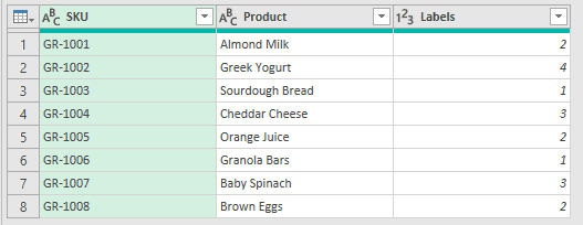
Below I have grocery SKUs, products, and Labels counts in A2:C9 on the Power Query Source sheet. I want each product repeated by its count.
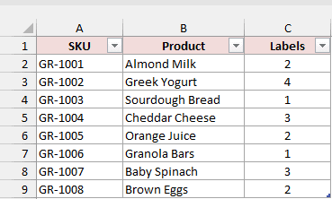
Here are the steps to repeat the rows using Power Query:
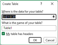
- Select any cell in the data, then go to the Data tab > From Table/Range. Power Query needs an Excel Table. If the Create Table dialog opens, keep “My table has headers” checked and click OK.
The Power Query Editor then opens with the data.
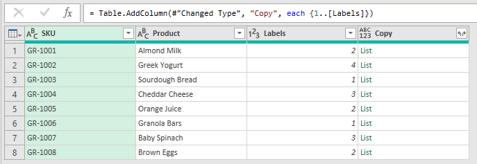
- Go to the Add Column tab > Custom Column. Set the new column name to Copy, enter the formula below, and click OK.
{1..[Labels]}
![The Custom Column dialog names the column Copy and uses = {1..[Labels]}, with no syntax errors detected.](https://spreadsheetplanet.com/wp-content/uploads/2026/10/rr-14-m5-custom-column-dialog.png)
This formula makes a list from 1 to that row’s Labels value. The new Copy column shows “List” in every cell.
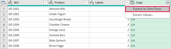
- Click the expand icon (two arrows) in the Copy header and choose Expand to New Rows.
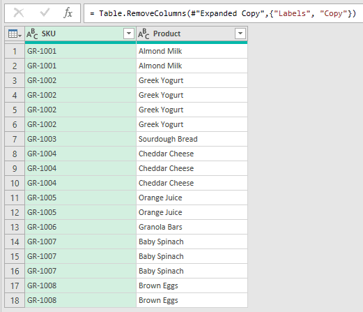
Each list item becomes its own row. A list containing 1 and 2 produces two copies of that product.
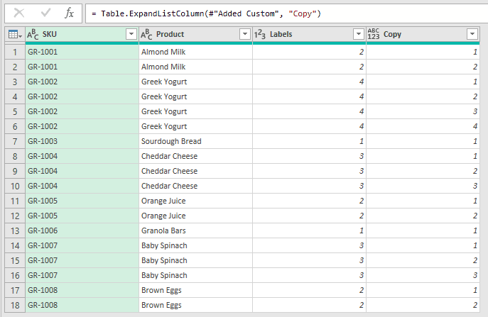
- Hold Ctrl, click the Labels and Copy headers, right-click one of them, and choose Remove Columns.
- Go to the Home tab > Close & Load.
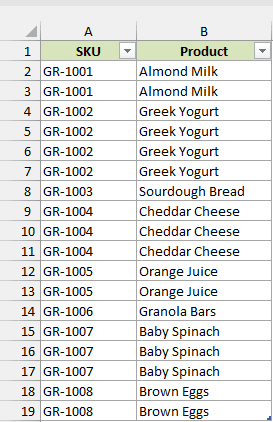
Power Query loads a new table with 18 rows onto a new sheet. The Power Query Result sheet shows the result, and the original data stays unchanged.
For a fixed count, use {1..3} instead of {1..[Labels]} to repeat every row three times.
When the source changes, update the output manually using Data > Refresh All.
Note: A Labels count of 0 creates an empty list, but Expand to New Rows still keeps one row for it. Filter out 0s in the Labels column before expanding.
Method #6: Using a VBA Macro
If you repeat rows often, or your Excel version has no CHOOSEROWS, a short macro can create the copies for you.
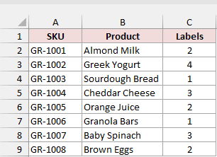
Below I have grocery SKUs, products, and Labels counts in A2:C9 on the VBA Macro sheet. I want each product repeated by its count.
Here is the VBA code:
Sub RepeatRows()
    Dim ws As Worksheet
    Dim lastRow As Long, r As Long, i As Long, outRow As Long

    Set ws = ActiveSheet
    lastRow = ws.Cells(ws.Rows.Count, "A").End(xlUp).Row

    ws.Range("E1:F1").Value = ws.Range("A1:B1").Value
    outRow = 2

    For r = 2 To lastRow
        For i = 1 To ws.Cells(r, "C").Value
            ws.Cells(outRow, "E").Resize(1, 2).Value = ws.Cells(r, "A").Resize(1, 2).Value
            outRow = outRow + 1
        Next i
    Next r
End SubHere are the steps to use this macro:
- Go to the data sheet and press Alt + F11 to open the VBA Editor.
- Choose Insert > Module.
- Paste the code above into the module.
- Put the cursor inside the code and press F5.
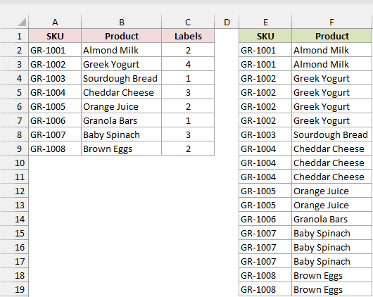
The result has headers in E1:F1 and 18 repeated rows in E2:F19.
The macro copies the headers to E1:F1, then writes each SKU and product as many times as column C specifies.
It finds the last source row by itself and skips rows with a 0 or blank count.
Note: Save the file as an Excel Macro-Enabled Workbook (.xlsm) to keep the macro. A regular .xlsx file drops it.
Additional Notes About Repeating Rows in Excel
Here’s a quick way to choose the method that fits what you need:
| What you need | Method to use |
|---|---|
| The whole list N times, once | Method #1 |
| Each row N times | Method #2 |
| The whole list repeated with a formula | Method #3 |
| Each row repeated by its own count | Method #4, #5, or #6 |
| An option without Microsoft 365 or Excel 2024 | Method #1, #5, or #6 |
- Leave empty cells below a formula so it has room to spill. Occupied cells can cause a #SPILL! error.
- Methods #2 to #4 update when the source changes. Power Query updates on refresh. Methods #1 and #6 produce fixed values.
- On Mac, use Command + C and Command + V. Open the VBA Editor with Option + F11, or Tools > Macro > Visual Basic Editor.
Frequently Asked Questions
Here are answers to a few other questions about repeating rows in Excel.
How do I repeat header rows on every printed page in Excel?
Use Print Titles, a different feature for printing. Go to Page Layout > Print Titles, then set Rows to repeat at top.
Can I repeat rows with a formula in older versions of Excel?
Enter this formula in D2, then fill it down 24 rows through D2:D25:
=INDEX($A$2:$A$9,ROUNDUP(ROWS($1:1)/$B$11,0))
It repeats each SKU by the count in B11. Use $B$2:$B$9 in place of $A$2:$A$9 in the next column for product names.
How do I turn the repeated rows into fixed values?
Copy the result, then right-click and choose Paste Special > Values.
Conclusion
I’ve shown you how to repeat individual rows, whole lists, and rows with different counts. I’d start with Method #2 for most tasks.
I hope you found this article helpful.
Other Excel articles you may also like:
- Table.ExpandListColumn Function (Power Query M)
- How to Insert Multiple Rows in Excel
- How to Loop in Excel Formulas Without VBA
- WRAPROWS Function in Excel
- How to Transpose Multiple Rows into One Column in Excel
- REPT Function in Excel
- How to Use the Fill Handle in Excel
- How to Convert Columns to Rows in Excel?
