
A dynamic named range in Excel is a name that grows with your data, so a formula, drop-down list, or chart that uses it picks up new rows automatically.
A normal named range doesn’t do that.
If SalesData points to B2:B9 and you add a sale in B10, the name still stops at B9, and your total quietly misses the new entry.
The fix is to define the name so Excel works out where the list ends every time it calculates.
In this article, I’ll show you how to build one with an Excel Table, TRIMRANGE, INDEX, and OFFSET, and then use it in a drop-down list and a chart.
Method #1: Naming an Excel Table Column
An Excel Table grows by itself when you add a row right below it. If you give one of its columns a defined name, that name grows with it.
Below I have the monthly online sales from January to August on the Table Method sheet.
I want a name that always covers every sales figure, including months I add later.
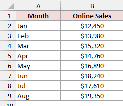
Here are the steps to turn the data into a Table and name its sales column:
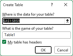
- Click any cell in the data and press Ctrl + T. In the Create Table dialog, keep My table has headers checked and click OK.
- On the Table Design tab, click in the Table Name box, type SalesTable, and press Enter.

- On the Formulas tab, click Define Name. In the New Name dialog, type SalesByTable in the Name box and enter this in the Refers to box:
=SalesTable[Online Sales]
![New Name dialog defining SalesByTable as =SalesTable[Online Sales].](https://spreadsheetplanet.com/wp-content/uploads/2026/09/dnr-04-m1-new-name.png)
- Click OK.
SalesTable[Online Sales] is a structured reference. It means “every data cell in the Online Sales column of SalesTable”, so the name follows the Table as it grows.
To test the name, here is the formula in E2:
=SUM(SalesByTable)
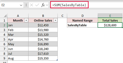
It returns $128,600, the total for January to August.
Now type Sep in A10 and 20150 in B10. The Table stretches to include the new row, and E2 changes to $148,750 without you touching the formula.
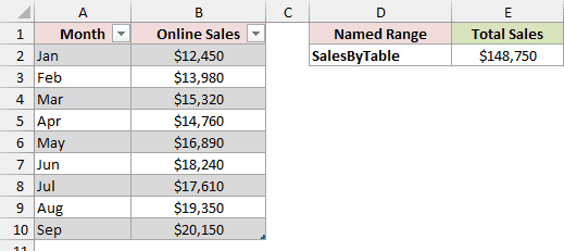
The Table does the growing here, and the name just points at it. That’s why I’d pick this method first.
There’s no formula to get wrong, and a blank cell in the middle of the list doesn’t break it.
Method #2: Using TRIMRANGE or a Trim Reference (Microsoft 365)
If you’re on Microsoft 365 and don’t want to convert your data to a Table, TRIMRANGE can do the job.
It takes a big range and trims off the empty rows around the data.
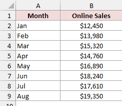
Below I have the same January to August sales, this time on the TRIMRANGE Method sheet as a plain range.
I want a name that covers only the filled sales cells.
Here are the steps to create the name:
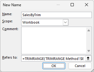
- On the Formulas tab, click Define Name. Type SalesByTrim in the Name box and enter this in the Refers to box:
=TRIMRANGE('TRIMRANGE Method'!$B$2:$B$1000)
- Click OK.
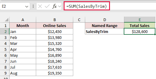
Here is the formula in E2 to check it:
=SUM(SalesByTrim)
How does this formula work?
B2:B1000 is far bigger than the data, so it leaves room for future months.
TRIMRANGE removes the empty rows before the first filled cell and after the last one, which leaves B2:B9 here.
SUM adds those eight cells and returns $128,600. Add September in row 10, and the trimmed range becomes B2:B10 on its own.
There’s also a shorter way to write this, called a trim reference.
Put a dot after the colon, and Excel trims the empty rows at the end of the range for you.
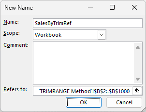
To try it, create a second name, SalesByTrimRef, the same way, with this in the Refers to box:
='TRIMRANGE Method'!$B$2:.$B$1000
Here is the formula in E3 to check it:
=SUM(SalesByTrimRef)
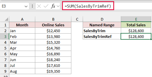
It returns the same $128,600. Both names behave the same way, so pick whichever one you find easier to read.
Note: TRIMRANGE and trim references are only available in Excel for Microsoft 365. Older versions don’t recognize them, so use Method #1 or Method #3 there.
Method #3: Using INDEX and COUNTA
This one works in every version of Excel, and it’s the one I’d use when the data has to stay a plain range.
INDEX finds the last filled cell, and the name runs from the first sale to that cell.
Below I have the monthly sales on the INDEX Method sheet. I want a defined name, SalesByIndex, that covers the sales in column B.
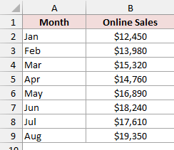
Here are the steps to create the name:
- On the Formulas tab, click Define Name. Type SalesByIndex in the Name box and enter this in the Refers to box:
='INDEX Method'!$B$2:INDEX('INDEX Method'!$B:$B,COUNTA('INDEX Method'!$B:$B))
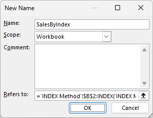
- Click OK.
Here is the formula in E2 to check it:
=SUM(SalesByIndex)
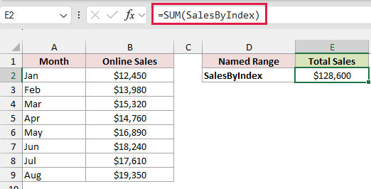
How does this formula work?
COUNTA counts the filled cells in column B. That’s 9 here, because it counts the Online Sales header along with the eight sales.
INDEX then returns the 9th cell of column B, which is B9. The colon joins B2 to that cell, so the name refers to B2:B9 and SUM returns $128,600.
Add September in B10, and COUNTA returns 10, so the name stretches to B2:B10.
Note: COUNTA only works if the column has no blank cells in the middle. If May were empty, COUNTA would come up one short, and the name would stop at B9 and miss September.
Method #4: Using OFFSET and COUNTA
OFFSET is the formula most older tutorials use for dynamic ranges, so you’ll probably run into it in workbooks you inherit.
Below I have the monthly sales on the OFFSET Method sheet. I want a defined name, SalesByOffset, that covers the sales in column B.
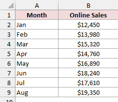
Here are the steps to create the name:
- On the Formulas tab, click Define Name. Type SalesByOffset in the Name box and enter this in the Refers to box:
=OFFSET('OFFSET Method'!$B$2,0,0,COUNTA('OFFSET Method'!$B:$B)-1,1)
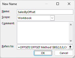
- Click OK.
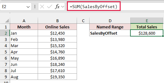
Here is the formula in E2 to check it:
=SUM(SalesByOffset)
How does this formula work?
OFFSET starts at B2 and moves 0 rows and 0 columns. The last two arguments set the size of the range: a height and a width of 1 column.
The height is COUNTA minus 1, which leaves out the header. That’s 8 here, so the name covers B2:B9 and SUM returns $128,600.
Why INDEX is usually the better choice
Both formulas return exactly the same range. The difference is when Excel recalculates them.
OFFSET is a volatile function. Excel recalculates it, and every formula that uses the name, whenever anything in the workbook changes.
INDEX isn’t volatile. It only recalculates when the cells it depends on change.
In a small file you won’t notice. In a big workbook with lots of formulas built on OFFSET names, it can make everything feel slow.
That’s why I’d use INDEX for new work.
Here’s how the four methods compare:
| Method | Works In | Recalculates on Every Change | Blank Cell Inside the List |
|---|---|---|---|
| Table column name | All current versions | No | Still covers every row |
| TRIMRANGE or trim reference | Microsoft 365 | No | Still reaches the last row |
| INDEX and COUNTA | All versions | No | Stops too early |
| OFFSET and COUNTA | All versions | Yes | Stops too early |
How to Use a Dynamic Named Range in a Drop-Down List and a Chart
A dynamic name pays off most where a fixed range would go stale. A drop-down list and a chart are the two most common places.
Below I have the INDEX Method sheet from Method #3, with the SalesByIndex name already set up.
I want a Pick a Month drop-down in G2 and a column chart of the sales.
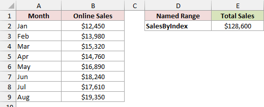
Both need the month names too, so first create a second name for column A.
- On the Formulas tab, click Define Name. Type MonthsByIndex in the Name box and enter this in the Refers to box, then click OK:
='INDEX Method'!$A$2:INDEX('INDEX Method'!$A:$A,COUNTA('INDEX Method'!$A:$A))
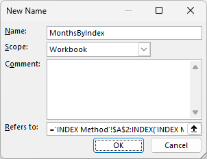
It’s the same formula as SalesByIndex, just pointed at column A.
Use the Name in a Drop-Down List
Here are the steps to create a drop-down list that grows with the months:
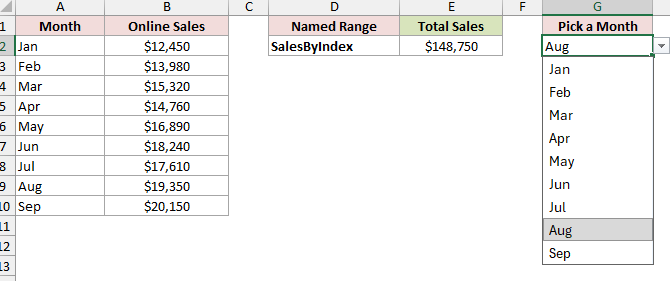
- Select G2. On the Data tab, click Data Validation. Choose List in the Allow box, type =MonthsByIndex in the Source box, and click OK.
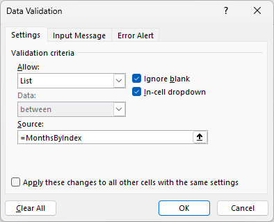
G2 now has a drop-down arrow that lists Jan to Aug.
If you used Method #1, type =SalesTable[Month] in the Source box and Excel won’t accept it, since Data Validation doesn’t take structured references.
Define a name for it instead, like MonthsByTable with =SalesTable[Month], and use =MonthsByTable as the source.
Use the Name in a Chart
A chart built on a normal range stays stuck on the months it started with.
When its series point to the names instead, new months show up in the chart as you add them.
Here are the steps to create the chart:
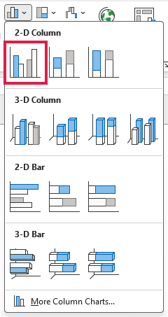
- Click an empty cell away from the data, such as I2. On the Insert tab, click Insert Column or Bar Chart and choose Clustered Column. Excel adds an empty chart.
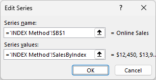
- Right-click the chart, choose Select Data, and click Add. Type =’INDEX Method’!$B$1 in the Series name box and =’INDEX Method’!SalesByIndex in the Series values box, then click OK.
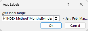
- Under Horizontal (Category) Axis Labels, click Edit. Type =’INDEX Method’!MonthsByIndex in the Axis label range box and click OK.
- Click OK to close the Select Data Source dialog.
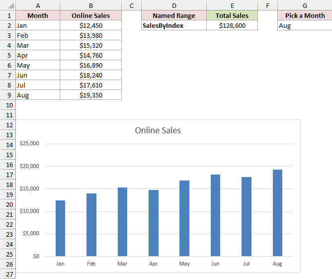
Note: The chart boxes need the sheet name in front of the defined name. If you type just =SalesByIndex, Excel rejects it. After you click OK, Excel swaps the sheet name for the file name, and that’s expected.
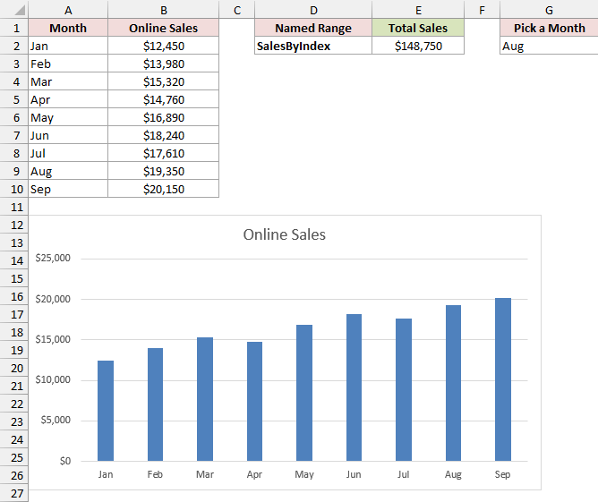
Now type Sep in A10 and 20150 in B10. The chart gets a ninth column, E2 changes to $148,750, and nothing else needs editing.
Click the arrow in G2, and Sep is in the drop-down list too.
If your data is a Table (Method #1), you don’t need names for the chart at all. A chart built straight from a Table already grows when the Table does.
The same goes for a PivotTable. Use the Table as its source, and after you add rows, click Refresh on the PivotTable Analyze tab to pull them in.
Additional Notes About Dynamic Named Ranges in Excel
- Keep other entries out of the column you’re counting. A note typed in B30 makes COUNTA one higher, so SalesByIndex runs one row past the last sale and your chart gets an empty column.
- If the column only holds numbers, you can use COUNT instead of COUNTA:
='INDEX Method'!$B$2:INDEX('INDEX Method'!$B:$B,COUNT('INDEX Method'!$B:$B)+1). COUNT skips the header and any stray text, and the +1 adds the header row back. - In Microsoft 365, a name can also point to a spill range, like
=$K$2#for the results of a UNIQUE formula in K2. It grows with the spill without any counting. - Names are workbook-wide by default, so each one needs a unique name. The Scope box in the New Name dialog can limit a name to a single sheet.
Frequently Asked Questions
Here are answers to a few common questions about dynamic named ranges.
How do I make a dynamic named range ignore blank cells?
TRIMRANGE (Method #2) already does this. It only trims empty rows at the top and bottom of the range, so a gap in the middle doesn’t cut it short.
In any version, you can use MATCH to find the last number instead of counting:
='INDEX Method'!$B$2:INDEX('INDEX Method'!$B:$B,MATCH(9.99E+307,'INDEX Method'!$B:$B))
9.99E+307 is bigger than any number in the column, so MATCH lands on the last number, even with blanks above it.
How can I see which cells a named range refers to?
Type the name in the Name Box to the left of the formula bar and press Enter. Excel selects the cells it refers to right now.
You can also open Formulas > Name Manager and select the name to see its formula in the Refers to box.
Can I create a dynamic named range with VBA?
Yes. Names.Add takes the same formula you’d type in the New Name dialog:
ActiveWorkbook.Names.Add Name:="SalesByIndex", _
RefersTo:="='INDEX Method'!$B$2:INDEX('INDEX Method'!$B:$B,COUNTA('INDEX Method'!$B:$B))"What are the rules for naming a range in Excel?
A name has to start with a letter, an underscore, or a backslash, and it can’t contain spaces. Sales_2025 and Sales.2025 both work, but Sales 2025 and 2025Sales don’t.
It also can’t look like a cell address. SAL2025 is rejected because SAL is a real column, and R and C are reserved on their own.
Conclusion
A dynamic named range saves you from editing ranges every time new data comes in.
If your data can be a Table, name a Table column. It’s the simplest option, and blank cells don’t trip it up.
For a plain range, go with INDEX and COUNTA in any version, or TRIMRANGE if you’re on Microsoft 365.
I hope you found this article helpful.
Other Excel articles you may also like:
