
If you add rows to a list every week, you’ll often need to know where the data ends.
Sometimes you just want to jump there. Other times you need that row number inside a formula.
Scrolling works for a short list. On a long sheet, it’s slow, and it’s easy to stop a few rows too early.
Blank cells are what make this tricky. A gap in the middle of a column makes the obvious shortcut stop early.
It also makes a simple count of filled cells come out too low.
In this article, I’ll show you six ways to find the last row with data, using keyboard shortcuts, Go To Special, and formulas built on XLOOKUP, LOOKUP, TRIMRANGE, and MAX.
Method #1: Using the Ctrl + Arrow Key Shortcuts
If you just want to see where your data ends, a keyboard shortcut is the fastest way to get there.
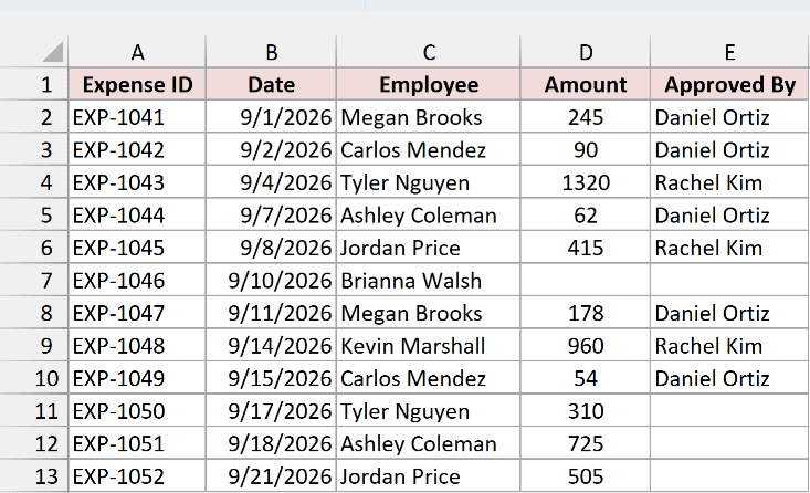
Below I have an expense log on the Expense Log sheet. Each row is one expense, and column D holds the amount.
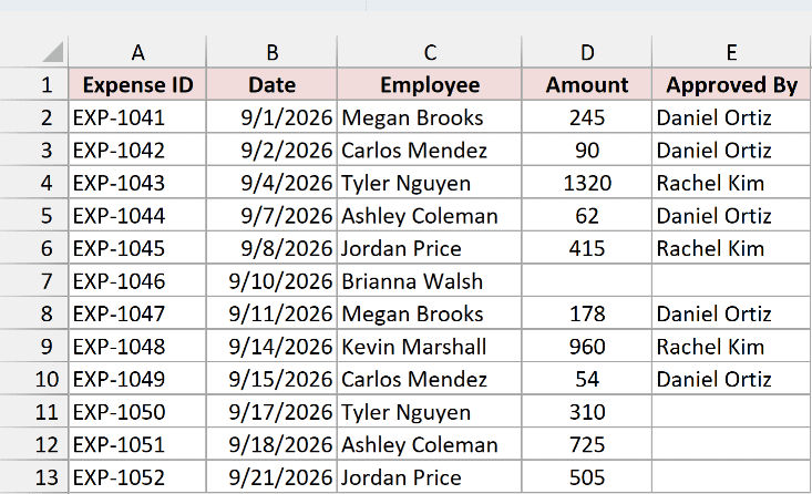
Expense EXP-1046 in row 7 doesn’t have an amount yet, so cell D7 is blank. I want to find the last row with data in column D.
Here are the steps to find it with the keyboard:
- Select cell D1 and press Ctrl + Down Arrow.
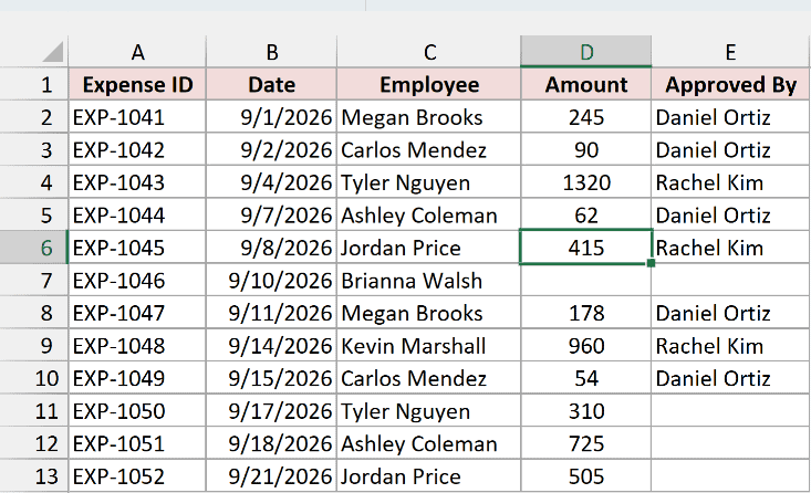
Excel stops at D6, not at the end of the list.
Ctrl + Down Arrow jumps to the last filled cell before a blank, so the empty D7 stops it early.
To get past the gap, start at the bottom of the column and come back up.
- Click in the Name Box (to the left of the formula bar), type D1048576, and press Enter.
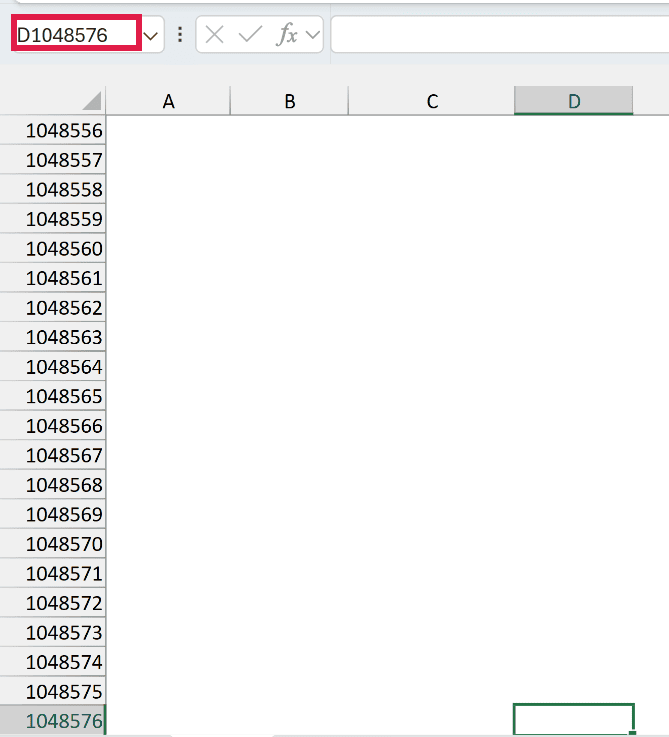
This takes you to the very last cell in column D. Row 1,048,576 is the last row on every Excel worksheet.
- Press Ctrl + Up Arrow.
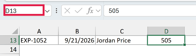
Excel jumps up to D13. The Name Box now shows D13, so the last row with data in column D is row 13.
Coming up from the bottom always works, because nothing sits below the last value to stop Excel on the way up.
On a Mac, use Command instead of Ctrl for these arrow key shortcuts.
Note: If your column has no blank cells, one Ctrl + Down Arrow from the top is enough. Add Shift (Ctrl + Shift + Down Arrow) to select everything down to that cell.
Method #2: Using the Go To Special Dialog Box
Here’s another way to do this. Go To Special has a Last cell option that jumps to the last used cell on the whole sheet, not just in one column.
Below I have the same expense log on the Expense Log sheet, with data from A1 to E13.
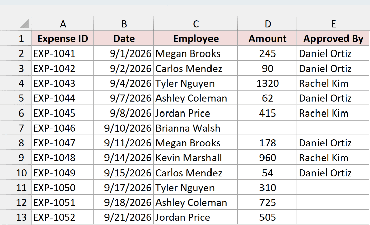
Expenses EXP-1050 to EXP-1052 haven’t been approved yet, so cells E11 to E13 are blank. I want the last row that has data anywhere on the sheet.
Here are the steps to use Go To Special:
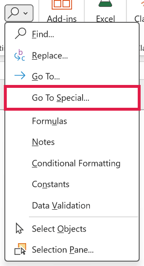
- On the Home tab, click Find & Select, then click Go To Special.
- In the Go To Special dialog box, select Last cell.
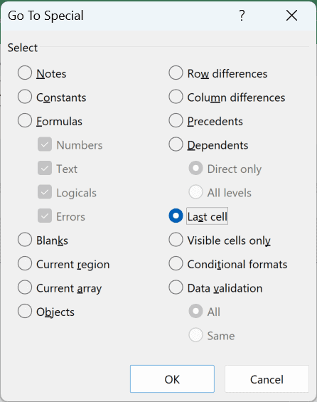
- Click OK.
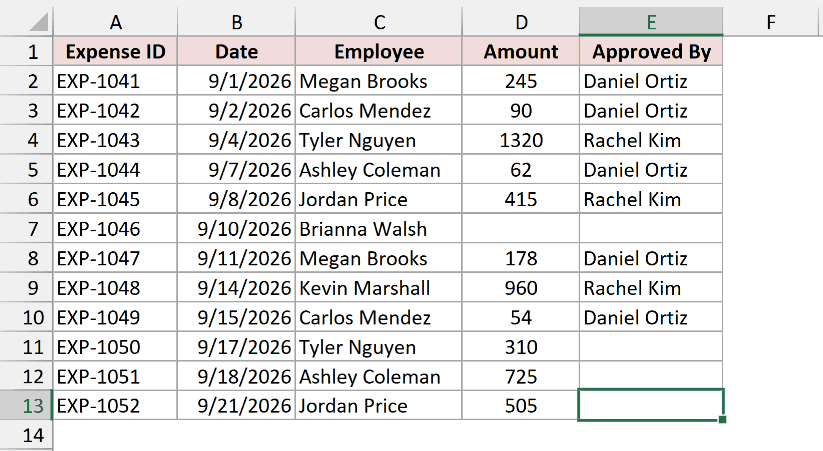
Excel selects E13. That’s where the last used row (13) meets the last used column (E).
Notice that E13 is blank. Last cell doesn’t look for a filled cell.
It goes to the corner of the area Excel treats as used, so read the row number, not the cell.
You can also press Ctrl + End to jump to the same cell without opening the dialog box.
Note: Last cell and Ctrl + End also count cells that only have formatting. If they land below your data, clear the formatting from those extra rows and save the workbook to reset it.
Method #3: Using the XLOOKUP Function
If you need the last row number inside a formula, so it updates as you add data, this is the method I’d use in Excel 365.
Below I have the same expense log on the Last Row Formulas sheet. The amounts are in column D, and cell D7 is blank.
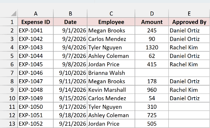
I want the row number of the last filled cell in column D, in cell H2.
Here is the formula:
=XLOOKUP(TRUE,D:D<>"",ROW(D:D),,0,-1)
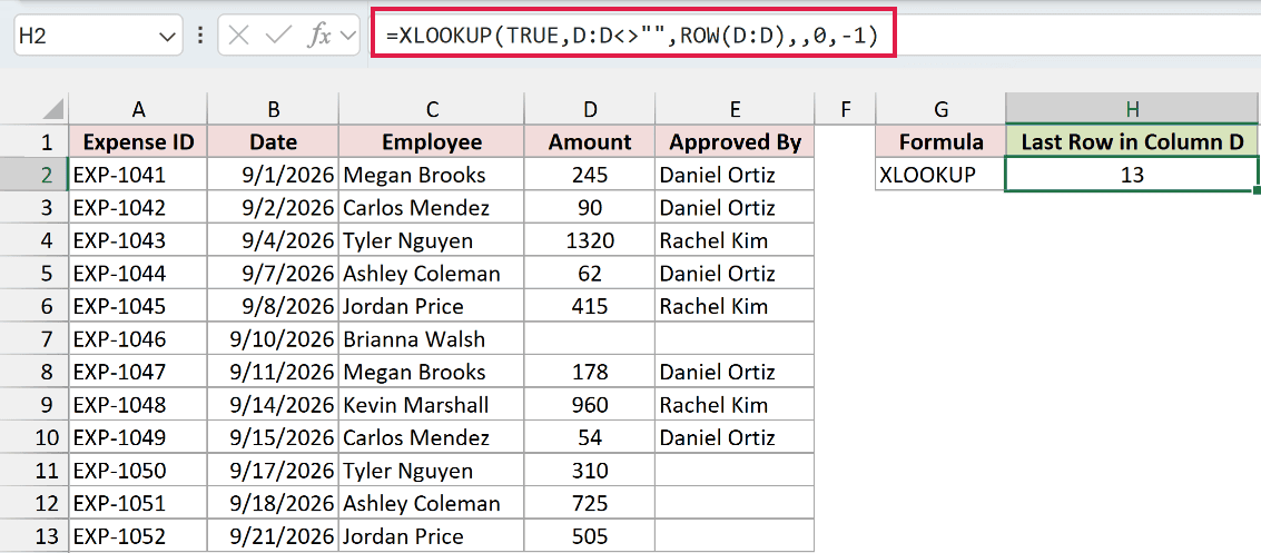
It returns 13, the last row with data in column D. The blank cell in D7 doesn’t throw it off.
How does this formula work?
D:D<>”” checks every cell in column D. It returns TRUE for a filled cell and FALSE for a blank one.
The ROW function returns a row number, so ROW(D:D) gives the row number of every cell in the column, from 1 to 1,048,576.
The XLOOKUP function looks for TRUE in the first list and returns the matching row number from the second. The 0 asks for an exact match.
The last argument, -1, is what makes it work. It tells XLOOKUP to search from the bottom up, so the first TRUE it finds is the last filled cell.
Because the formula looks at the whole column, the result changes as soon as you add a row. Type an amount in D14 and it returns 14.
Note: XLOOKUP is available in Excel 2021, Excel 2024, and Microsoft 365. In older versions, use the LOOKUP formula in the next method.
Method #4: Using the LOOKUP Function
If you’re on Excel 2019 or older, you won’t have XLOOKUP. This LOOKUP formula does the same job and works in every version of Excel.
Below I have the expense log on the Last Row Formulas sheet. The amounts are in column D, with a blank cell in D7.
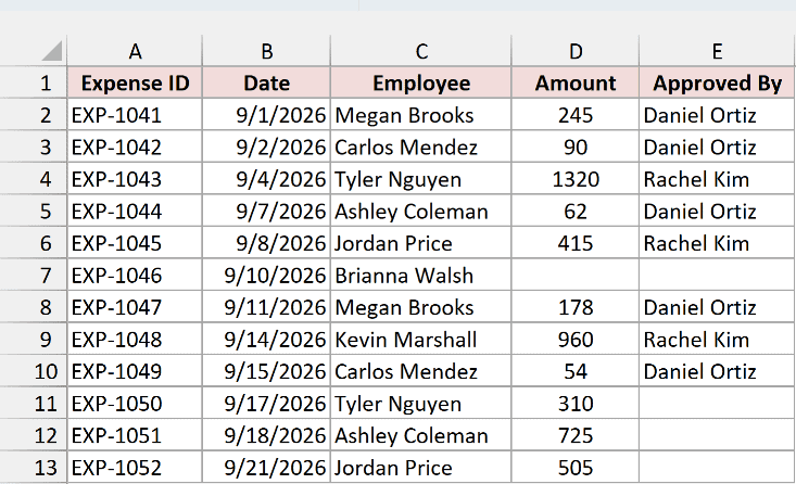
I want the last row with data in column D, in cell H3.
Here is the formula:
=LOOKUP(2,1/(D:D<>""),ROW(D:D))
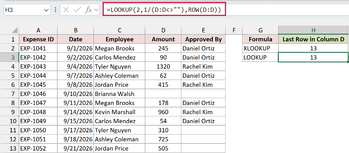
It returns 13, the same answer as XLOOKUP.
How does this formula work?
D:D<>”” returns TRUE for each filled cell in column D and FALSE for each blank one.
Excel treats TRUE as 1 and FALSE as 0. So 1/(D:D<>””) turns every filled cell into 1 and every blank cell into a #DIV/0! error.
The LOOKUP function then looks for 2 in that list. It can’t find one, since every value is either 1 or an error.
When the lookup value is bigger than everything in the list, LOOKUP matches the last number it finds and skips the errors.
That’s the last 1, which belongs to the last filled cell.
ROW(D:D) is the list LOOKUP returns from, so it returns the row number at that position, which is 13.
You don’t need Ctrl + Shift + Enter here, even in older versions, because LOOKUP works with arrays on its own.
Method #5: Using the TRIMRANGE Function
Microsoft 365 has a newer function made for this kind of job. TRIMRANGE removes the empty rows from the end of a range, so you can count what’s left.
Below I have the expense log on the Last Row Formulas sheet. The amounts are in column D, and D7 is blank.
I want the last row with data in column D, in cell H4.
Here is the formula:
=ROWS(TRIMRANGE(D:D,2))
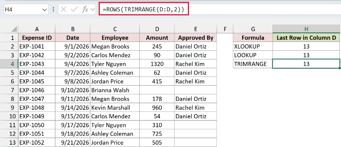
It returns 13.
How does this formula work?
The TRIMRANGE function takes all of column D and trims the empty rows from the end. The 2 tells it to trim trailing rows only, so it returns D1:D13.
Blank cells in the middle, like D7, stay in the range. Only the empty rows after the last value get removed.
The ROWS function then counts the rows in D1:D13, which is 13.
That count equals the row number only because the range starts in row 1. For a range like D2:D100, add 1 to the result to get the row number.
You can also write this with a trim reference, =ROWS(D:.D).
The dot after the colon tells Excel to trim the empty cells at the end, the same as TRIMRANGE with 2.
Note: TRIMRANGE and trim references are only available in Microsoft 365. Older versions of Excel don’t support either one, so use Method #3 or Method #4 there.
Method #6: Using MAX and ROW (Across Multiple Columns)
The methods so far find the last row in one column. Sometimes your columns have different lengths, and you want the last row with data in any of them.
Below I have three team lists on the Team Roster sheet, with Marketing in column A, Sales in column B, and Support in column C.
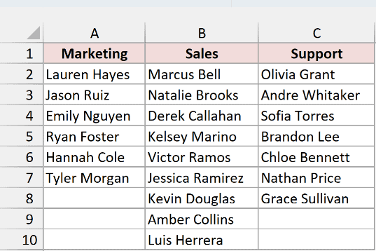
Each list has a different number of names. I want the last row that has data in any of the three columns, in cell E2.
Here is the formula:
=MAX((A:C<>"")*ROW(A:C))
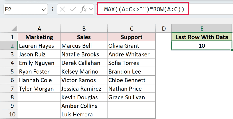
It returns 10. The Sales list in column B is the longest, and it ends in row 10.
How does this formula work?
A:C<>”” checks every cell in columns A to C. It returns TRUE for a filled cell and FALSE for a blank one.
Multiplying by ROW(A:C) turns each TRUE into its row number and each FALSE into 0.
The MAX function then returns the largest number in that grid. That’s the last row with data in any of the three columns.
You don’t need to know which list is the longest. Add a name to the bottom of any column, and the result moves down with it.
Note: In Excel 2019 and older, press Ctrl + Shift + Enter instead of Enter to confirm this formula. In Excel 2021 and Microsoft 365, Enter is enough.
Additional Notes About Finding the Last Row With Data in Excel
- Counting filled cells gives the wrong row when there are blanks. =COUNTA(D:D) returns 12 on the Last Row Formulas sheet, because it counts filled cells. The real last row is 13, since D7 is blank.
- Formulas that return an empty string are handled differently. A cell with a formula like =”” looks blank. Methods #3, #4, and #6 treat it as blank, but TRIMRANGE counts it as data.
- Whole-column references can slow down big workbooks. Method #6 checks over three million cells. If your sheet is heavy, use a fixed range like A1:C5000 instead of A:C.
- In a macro, the Ctrl + Up Arrow trick has a code version. To find the last row using VBA, use Cells(Rows.Count, “D”).End(xlUp).Row, which starts at the bottom of column D and moves up.
Frequently Asked Questions
Here are answers to a few questions people often ask about finding the last row in Excel.
How do I get the last value in a column instead of the row number?
Change the third argument of the XLOOKUP formula from ROW(D:D) to D:D: =XLOOKUP(TRUE,D:D<>””,D:D,,0,-1). On the Last Row Formulas sheet, it returns 505.
If you need the last value that matches a condition, like the last expense for one employee, see how to find the last occurrence of a value in a column.
How do I find the last column with data in a row?
Swap the column reference for a row reference, and swap ROW for the COLUMN function. =XLOOKUP(TRUE,1:1<>””,COLUMN(1:1),,0,-1) returns 5 on the Expense Log sheet, because the headers end in column E.
Do these formulas update when I add new rows?
Yes. Methods #3 to #6 look at whole columns, so a value typed below the current data is picked up right away.
The keyboard shortcuts and Go To Special only show where the data ends at that moment.
Conclusion
In this article, I showed you six ways to find the last row with data in Excel.
They range from the Ctrl + Arrow shortcuts and Go To Special to formulas with XLOOKUP, LOOKUP, TRIMRANGE, and MAX.
For most people, the XLOOKUP formula is the one to reach for, since it handles gaps and updates as you add rows.
I hope you found this article helpful.
Other Excel articles you may also like:
