
A dynamic top 10 list in Excel pulls the ten highest values out of your data and keeps itself current, so when a number changes, the ranking changes with it. Think of a sales leaderboard that reshuffles the moment someone closes a big deal.
Sorting the data by hand gets you a top 10 once. The trouble is that it goes stale the next time anyone edits a number.
Ties make it trickier too, because two people can share 10th place and you have to decide whether both make the list.
In this article, I’ll show you four ways to build one, using TAKE with SORT, FILTER with LARGE, a LARGE and INDEX setup for older Excel versions, and a Pivot Table with a Top 10 filter.
Method #1: Using the TAKE and SORT Functions
This is the method I’d use if you have Microsoft 365 or Excel 2024. One formula sorts the data from highest to lowest and keeps the first ten rows, and the result updates on its own whenever the data changes.
Below I have a dataset with 18 sales reps, their region, and their Q3 revenue. I want a list of the top 10 reps by revenue, with all three columns.
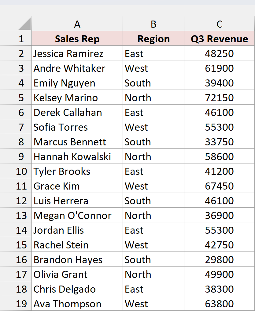
Here is the formula I entered in cell E2:
=TAKE(SORT(A2:C19,3,-1),10)
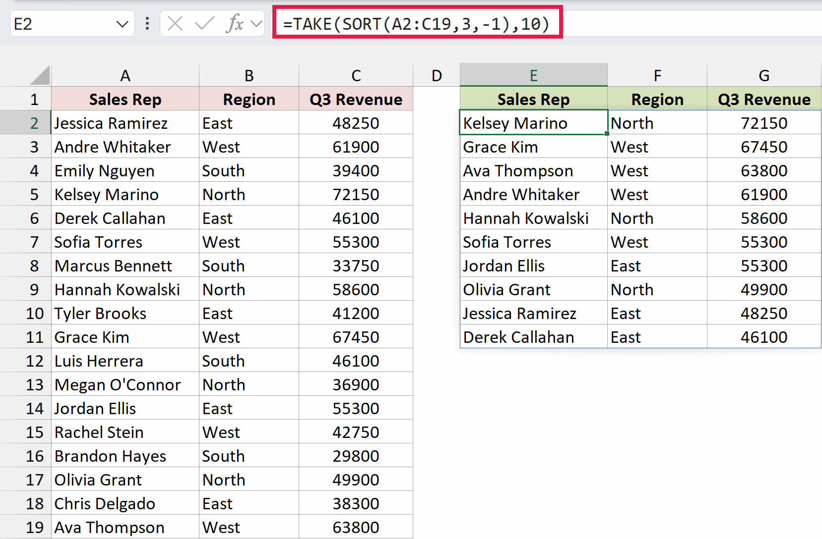
The formula spills down and across automatically, so you only enter it in one cell. I typed the headers in E1:G1 myself, since the formula returns only the data rows.
How does this formula work?
SORT sorts the whole range A2:C19 by its third column (Q3 Revenue). The -1 tells it to sort in descending order, so the highest revenue ends up on top.
TAKE then keeps the first 10 rows of that sorted result and drops the rest.
Ties need a closer look, though. Derek Callahan and Luis Herrera both have 46,100, which ties them for 10th place.
SORT keeps tied rows in their original order, so Derek (who comes first in the data) makes the list and Luis doesn’t. If you’d rather include everyone who’s tied, Method #2 handles that.
To see the list update, I changed Brandon Hayes’ revenue in C16 from 29,800 to 70,000.
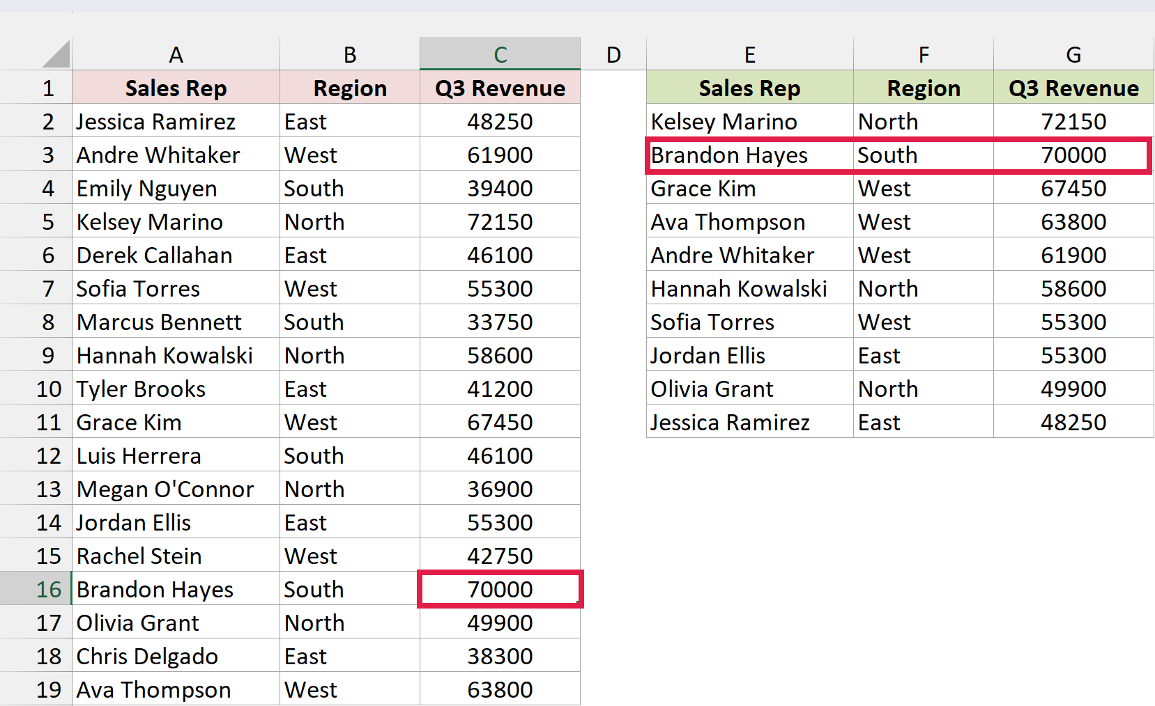
Brandon jumps straight to the #2 spot, and Derek Callahan drops off the list. I didn’t have to touch the formula. It recalculates the moment the data changes.
You can also make the number of rows adjustable. Instead of hard-coding 10, I typed 5 in cell I2 (under a Top N header) and pointed the formula to it:
=TAKE(SORT(A2:C19,3,-1),I2)
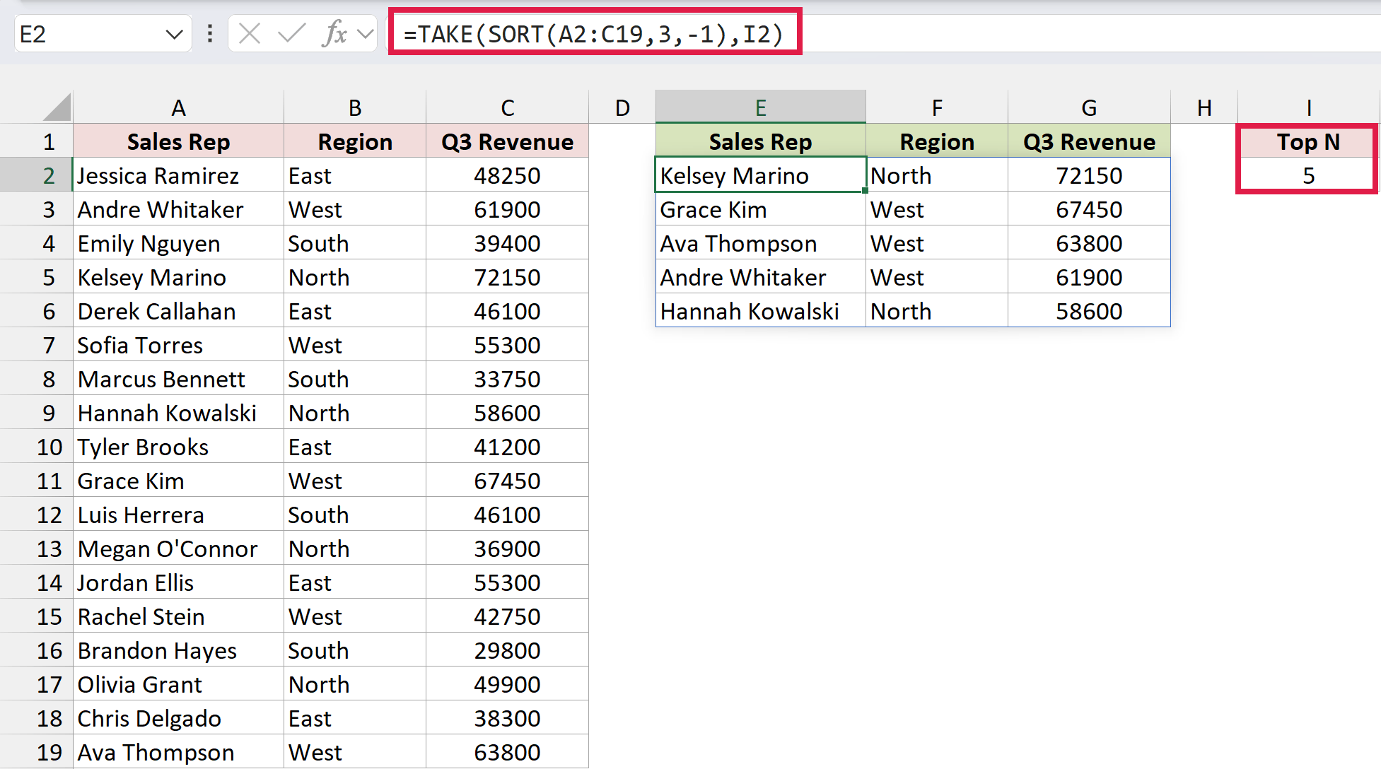
Now the list shows the top 5. Change I2 to 10, 3, or 15, and the list resizes to match.
Note: TAKE isn’t available in Excel 2021. If that’s your version, =INDEX(SORT(A2:C19,3,-1),SEQUENCE(10),{1,2,3}) returns the same ten rows. SEQUENCE(10) picks rows 1 to 10 of the sorted data, and {1,2,3} picks all three columns.
Method #2: Using FILTER and LARGE (Keeps Ties)
Here’s another way to do it, and this one treats ties differently. Instead of cutting the list at exactly ten rows, it keeps every row whose value is at least as high as the 10th-highest value.
Below I have the same dataset with 18 sales reps, their region, and their Q3 revenue. I want the top 10 reps by revenue, and if two reps tie for 10th place, I want both of them on the list.
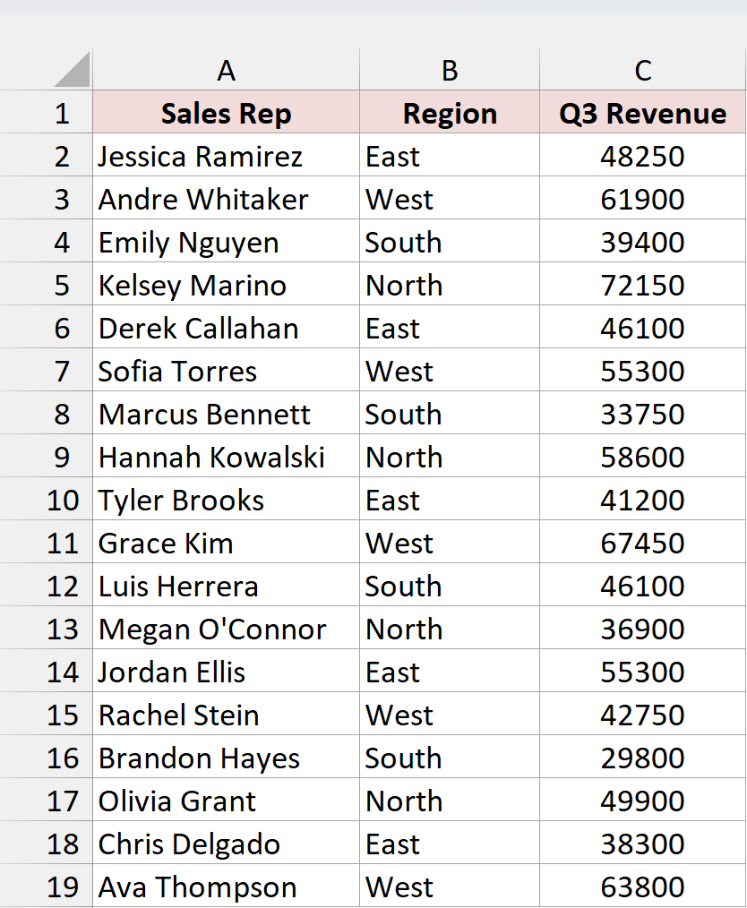
Here is the formula I entered in cell E2:
=SORT(FILTER(A2:C19,C2:C19>=LARGE(C2:C19,10)),3,-1)
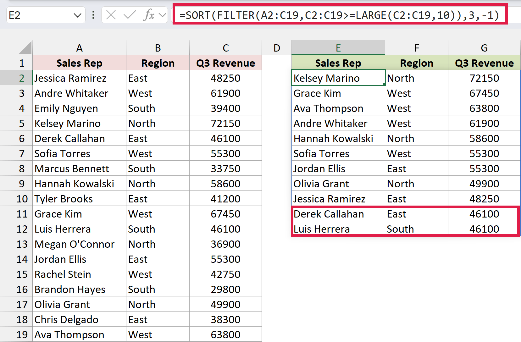
This time the list has 11 rows. Derek Callahan and Luis Herrera are tied at 46,100 for 10th place, so both of them are included.
How does this formula work?
LARGE(C2:C19,10) returns the 10th-highest revenue in the column, which is 46,100.
FILTER then keeps every row where the revenue is greater than or equal to 46,100. Because two reps share that value, 11 rows pass the test.
Finally, SORT puts those rows in descending order of revenue (column 3, -1), so the list reads from highest to lowest.
FILTER and SORT work in Excel 2021, Excel 2024, and Microsoft 365. Like Method #1, the list updates on its own when the revenue numbers change.
Method #3: Using LARGE, INDEX, and AGGREGATE (Older Versions)
If you’re on Excel 2019 or earlier, there’s no SORT, FILTER, or TAKE. You can still build a dynamic top 10, but it takes two formulas, each copied down ten rows.
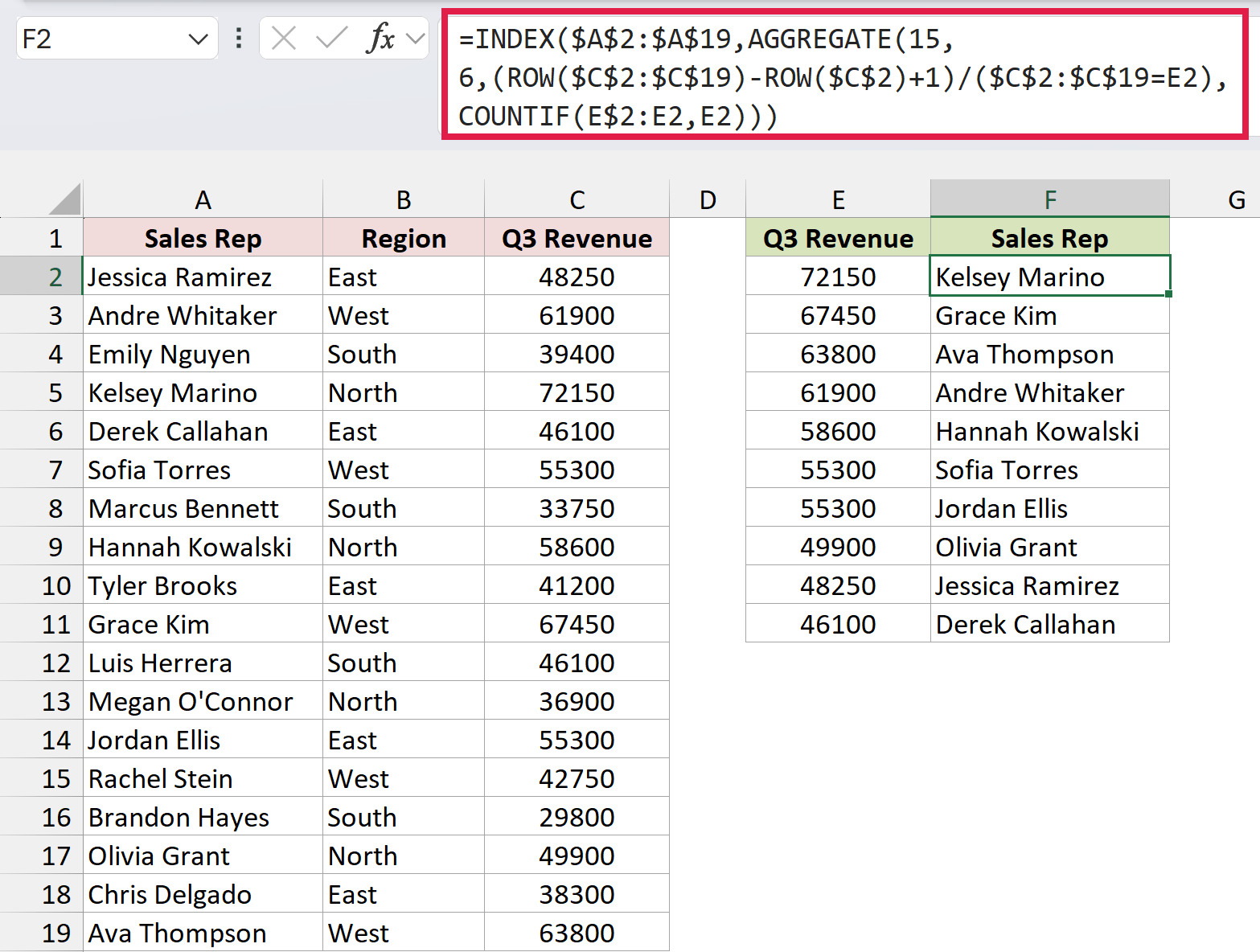
Below I have the same dataset with 18 sales reps, their region, and their Q3 revenue. I want the top 10 revenue figures along with the name of the rep for each one.
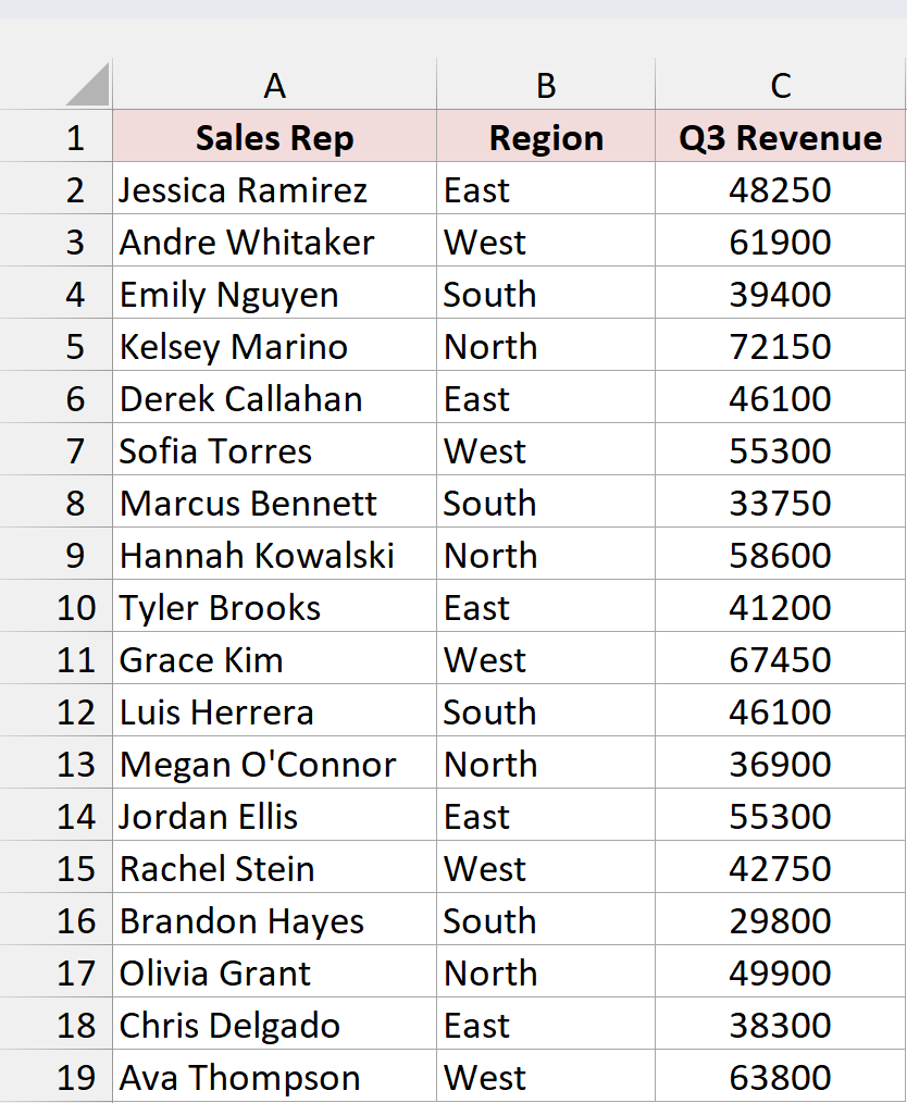
First, I’ll get the top 10 revenue values. Here is the formula I entered in cell E2 and copied down to E11:
=LARGE($C$2:$C$19,ROWS(E$2:E2))
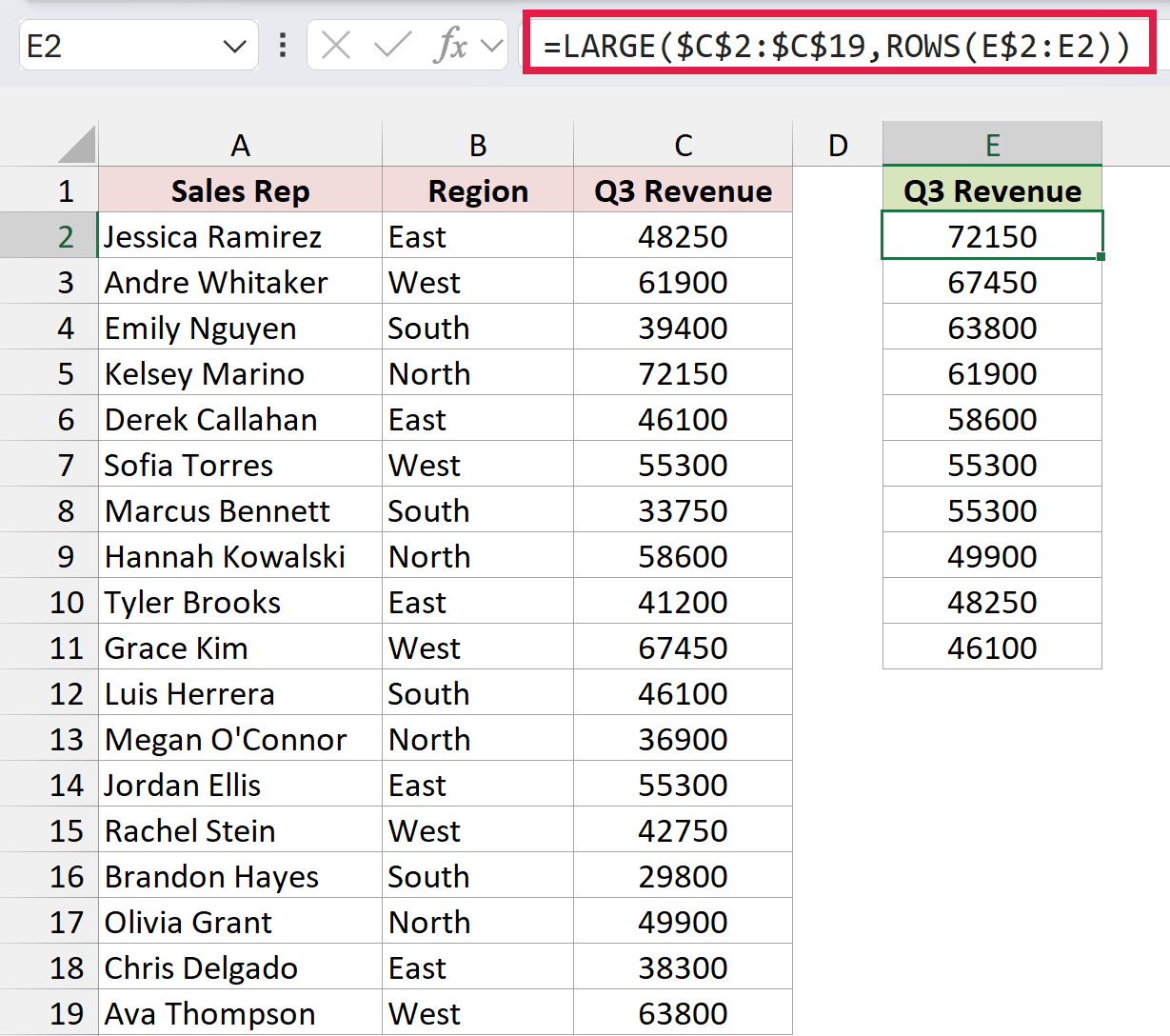
ROWS(E$2:E2) returns 1 in the first cell. As you copy the formula down, the range grows to E$2:E3, E$2:E4, and so on, so it returns 2, 3, and up to 10. That makes LARGE return the 1st, 2nd, 3rd, and up to the 10th-highest revenue.
Next, I need the rep name for each value. Here is the formula I entered in cell F2 and copied down to F11:
=INDEX($A$2:$A$19,AGGREGATE(15,6,(ROW($C$2:$C$19)-ROW($C$2)+1)/($C$2:$C$19=E2),COUNTIF(E$2:E2,E2)))
How does this formula work?
The usual way to look up a name is INDEX with MATCH. The problem is ties. Sofia Torres and Jordan Ellis both have 55,300, and MATCH always returns the first match, so you’d see Sofia’s name twice and Jordan would never show up.
AGGREGATE fixes that. The part (ROW($C$2:$C$19)-ROW($C$2)+1) returns the position of each row (1 to 18). Dividing it by ($C$2:$C$19=E2) keeps the positions where the revenue matches E2 and turns every other position into a #DIV/0! error.
AGGREGATE with 15 (SMALL) and 6 (ignore errors) then picks from the positions that are left. COUNTIF(E$2:E2,E2) tells it which one to pick. It counts how many times the current value has appeared so far in the list.
For the first 55,300 (in E7), COUNTIF returns 1, so AGGREGATE picks Sofia’s position. For the second 55,300 (in E8), it returns 2, so it picks Jordan’s. Finally, INDEX returns the name at that position.
To also pull the region, copy the same formula into the next column and change $A$2:$A$19 to $B$2:$B$19. This method works in Excel 2010 and later, and both formulas recalculate when the revenue changes.
Method #4: Using a Pivot Table With a Top 10 Filter
If you’d rather not write formulas at all, a Pivot Table has a built-in Top 10 filter. The one difference is that a Pivot Table doesn’t update by itself. You need to refresh it after the data changes.
Below I have the same dataset with 18 sales reps, their region, and their Q3 revenue. I want a Pivot Table that shows only the top 10 reps by revenue, sorted from highest to lowest.
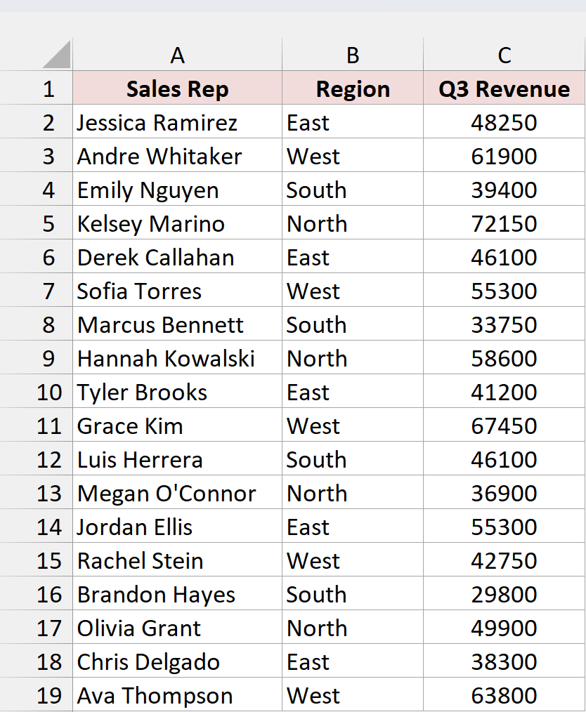
Here are the steps to create a top 10 list with a Pivot Table:
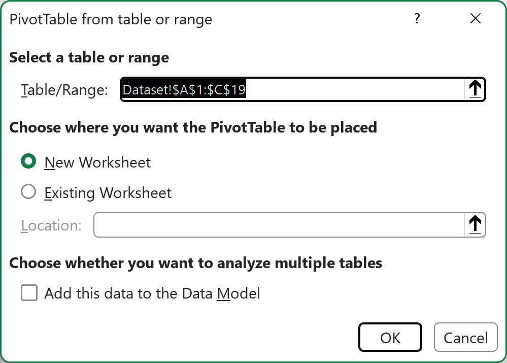
- Select the data (A1:C19), go to the Insert tab, and click PivotTable. In the dialog box that opens, keep New Worksheet selected and click OK.
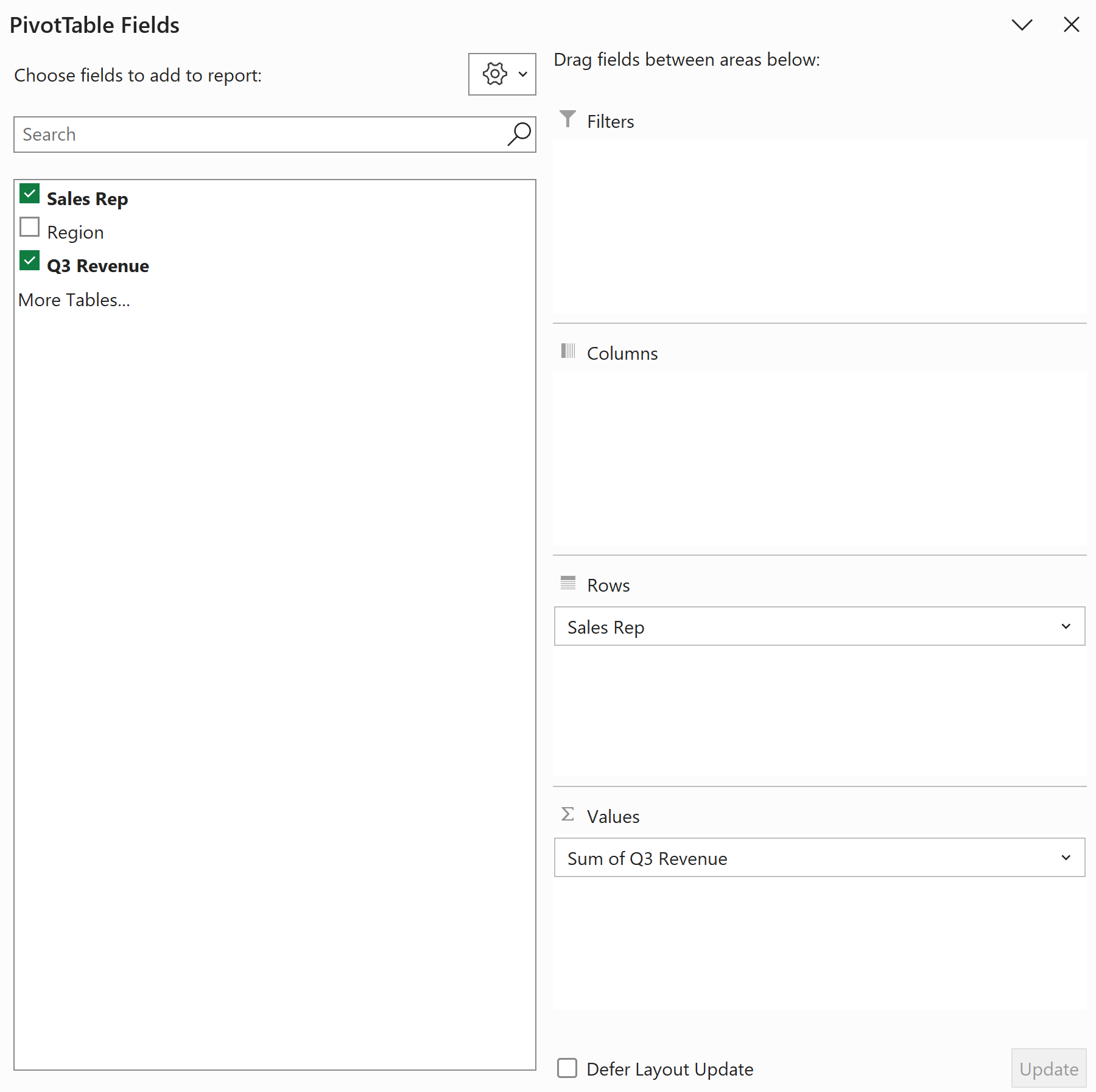
- In the PivotTable Fields pane, check Sales Rep so it goes into the Rows area, and check Q3 Revenue so it goes into the Values area as Sum of Q3 Revenue.
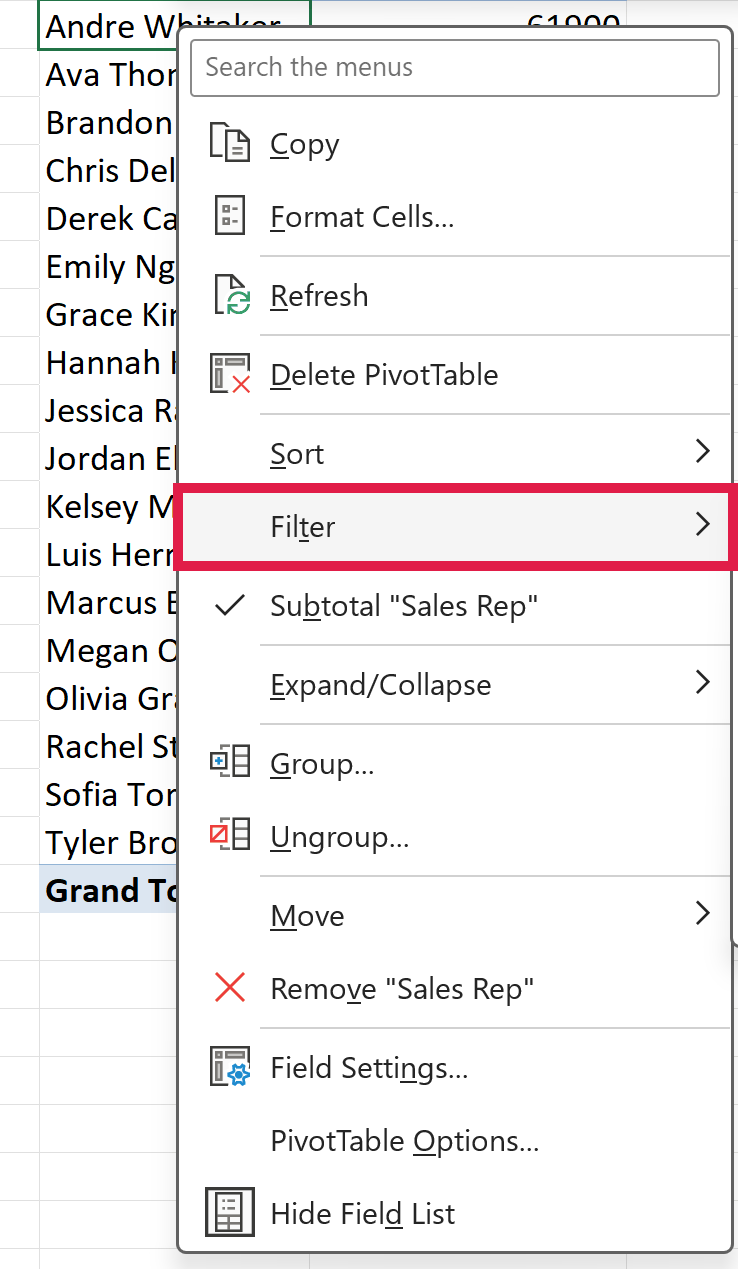
- Right-click any rep name in the Pivot Table, go to Filter, and click Top 10.
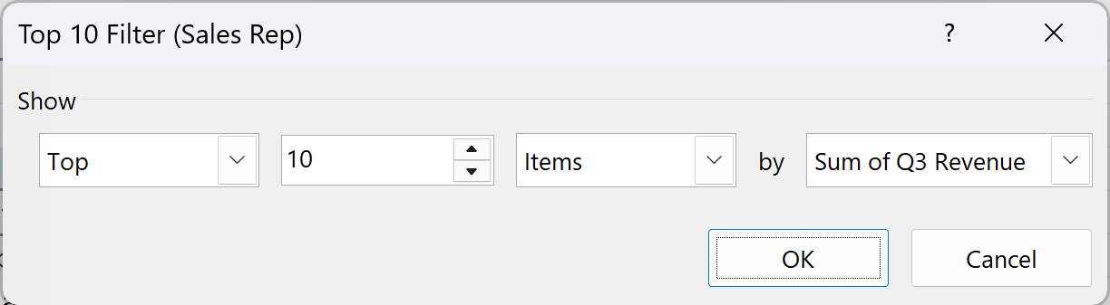
- In the Top 10 Filter dialog box, keep the settings as Top, 10, Items, by Sum of Q3 Revenue, and click OK.
- Right-click any revenue value in the Pivot Table, go to Sort, and click Sort Largest to Smallest.
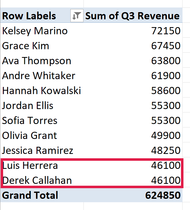
The Pivot Table now shows the top reps sorted from highest to lowest. Just like Method #2, it includes both Derek Callahan and Luis Herrera because they’re tied for 10th place, so you get 11 names.
When the revenue numbers change, right-click anywhere in the Pivot Table and click Refresh (or go to Data > Refresh All). The Top 10 filter and the sort order stay in place and apply to the new numbers.
Note: The Top 10 Filter dialog box isn’t limited to 10. You can change the number to show the top 5 or top 20, or switch Top to Bottom to show the lowest values instead.
Additional Notes About Creating a Dynamic Top 10 List in Excel
- Decide how you want to handle ties. TAKE with SORT always returns exactly 10 rows, so a tied rep can get left out. FILTER with LARGE and the Pivot Table’s Top 10 filter include every tied row, so the list can run longer than 10.
- Formulas update instantly, but a Pivot Table doesn’t. The three formula methods recalculate as soon as a number changes. A Pivot Table only shows new numbers after you refresh it.
- If you add new rows, use an Excel Table. A range like A2:C19 won’t pick up a new rep added in row 20. Convert the data to a Table (Ctrl + T), and the formulas and the Pivot Table’s source grow with it.
- AutoFilter and conditional formatting don’t build a list. Both have a Top 10 option, but AutoFilter only hides the other rows in place, and conditional formatting only highlights the top values. Neither gives you a separate, sorted top 10 list.
Frequently Asked Questions
Here are some questions people often ask about building a top 10 list in Excel.
How do I get the bottom 10 instead of the top 10?
Change the sort order in the TAKE formula from -1 to 1, so it reads =TAKE(SORT(A2:C19,3,1),10). That sorts from lowest to highest, so the first ten rows are the lowest ten. In the older-version method, use SMALL instead of LARGE.
How do I make a top 10 list for each region?
Filter the data for one region before sorting. For example, =TAKE(SORT(FILTER(A2:C19,B2:B19=”West”),3,-1),3) returns the top 3 reps in the West region. Point the “West” part at a cell, and you can switch regions from a single cell.
Why does my top 10 list show 11 names?
That happens when two or more values tie for 10th place and you’re using FILTER with LARGE or a Pivot Table Top 10 filter. Both include every tied row. If you need exactly 10 rows, use TAKE with SORT instead.
Can I show the top 10 percent instead of the top 10 items?
Yes. Swap LARGE for PERCENTILE.INC in the FILTER formula: =SORT(FILTER(A2:C19,C2:C19>=PERCENTILE.INC(C2:C19,0.9)),3,-1). PERCENTILE.INC(C2:C19,0.9) returns the 90th percentile (64,895 here), so only the two reps above it make the list.
Be careful with the Percent option in a Pivot Table’s Top 10 filter. It keeps the biggest items until they add up to 10% of the grand total. That’s a different rule, even when it lands on the same names.
Conclusion
In this article, I showed you four ways to create a dynamic top 10 list in Excel: TAKE with SORT, FILTER with LARGE, LARGE with INDEX and AGGREGATE for older versions, and a Pivot Table with a Top 10 filter.
If you have Microsoft 365 or Excel 2024, I’d go with TAKE and SORT. It’s one short formula, and it always returns exactly ten rows. I hope you found this article helpful.
Other Excel articles you may also like:
- How to Sort by Column in Excel (5 Easy Ways)
- INDEX MATCH Return Multiple Values in Excel (4 Easy Ways)
- RANK Function in Excel
- How to Create a Dynamic Named Range in Excel (4 Easy Ways)
- How to Use Structured References in Excel (6 Easy Ways)
- CHOOSEROWS Function in Excel
- SMALL Function in Excel
- SORTBY Function in Excel