Some Excel users have a need to show the subscript in some cells.
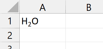
For example, if you want to write H2O in Excel, where you want the 2 to be below the H and the O, you will have to format it as a subscript.

While there is no option in the Excel ribbon to do this, you can still do this by going to the Format Cells dialog box. And you can also use a keyboard shortcut.
In this tutorial, I will give you the shortcut to apply a subscript format in Excel.
Shortcut to Subscript in Excel
Adding a subscript in Excel is a two-step step process:
First, you need to open the Format Cells dialog Box (which can be done with the below shortcut):
Control + 1
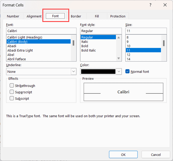
And then, you need to select the Subscript option (once you’re in the Font tab). This can be done using the below shortcut.
ALT + B + Enter
How to Use the Keyboard Shortcut to Subscript in Excel
Below are the steps to use the above keyboard shortcut:
- Select the cell on which you want to apply the subscript format
- Use the keyboard shortcut Control + 1 (hold the control key and then press the 1 key)
- In the Format Cells dialog box, select the Font tab

- Use the keyboard shortcut ALT + B + Enter (press in succession)
Important Things to Know About Subscript in Excel:
In most cases, you would be required to apply the Subscript format only to a portion of the text in a cell (rather than the entire cell)
To do this, place your cursor inside the cell and select the text on which you want to apply the subscript format, and then follow the steps above
Pro Tip: If you need to alley the subscript format quite often you can add the subscript icon in the quick access toolbar so that you can access it with a single click
Other Excel shortcuts you may also like:
- Excel Keyboard Shortcuts
- Wrap Text in Excel (Shortcut)
- Insert Hyperlink in Excel (Shortcut)
- Add Comments in Excel (Shortcut)
- Center Align in Excel (Shortcut)
- Superscript in Excel (Shortcut)\
- Insert Checkmark in Excel (Shortcut)
Other Excel Tutorials You May Also Like:
