If you want to get the average of only the cells that meet a condition, the AVERAGEIF function does that in a single step.
You give it a range to check, a condition to match, and the cells you want to average.
In this tutorial I’ll walk you through the syntax and five practical examples. AVERAGEIF returns a single value, but it composes with dynamic arrays.
AVERAGEIF Function Syntax in Excel
Here is what the AVERAGEIF function looks like:
=AVERAGEIF(range, criteria, [average_range])
- range = the cells checked against the criteria
- criteria = the condition (a number, text like “West”, an expression like “>100” in quotes, or a wildcard like “A*”)
- [average_range] (optional) = the cells actually averaged; if omitted, range is averaged
If you leave out average_range, AVERAGEIF averages the same cells it checks. The function returns a #DIV/0! error if no cells match the criteria. Matching is case-insensitive, so “west” and “West” are treated the same.
When to Use the AVERAGEIF Function
- You want to average sales, scores, or amounts for a single category, region, or status.
- You need the average of values above or below a threshold.
- You want to match a group of items using a wildcard (like all names starting with “A”).
- You want a quick one-condition average before stepping up to AVERAGEIFS for multiple criteria.
- You are already using SUMIF or COUNTIF and need a matching per-category average to go alongside.
Example 1: Average Sales by Region
Let’s start with a common scenario: averaging sales for one region.
The data has Rep names in column A, Region in column B, and Sales in column C, across rows 2 to 8.
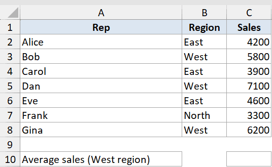
You want to find the average sales amount for the West region only.
Here is the formula:
=AVERAGEIF(B2:B8,"West",C2:C8)
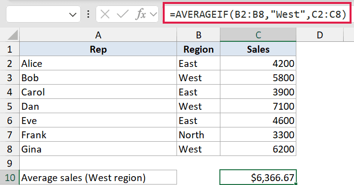
This returns 6366.67, the average of Bob (5800), Dan (7100), and Gina (6200).
The first argument is the range you check (Region), and the third is the range you average (Sales). AVERAGEIF lines them up row by row and only averages the Sales values where Region equals “West”.
Example 2: Average Orders Above a Threshold
Here’s another practical scenario: averaging only the orders that clear a cutoff.
The data has Order IDs in column A and Amount in column B, across rows 2 to 8.
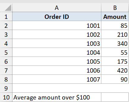
You want to find the average amount for orders over $100.
Here is the formula:
=AVERAGEIF(B2:B8,">100")
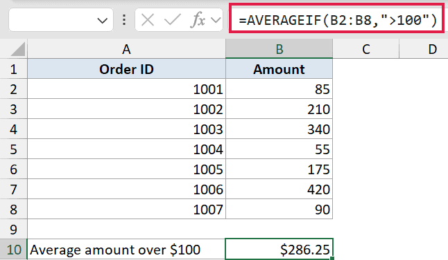
This returns 286.25. The operator and number go inside quotes as “>100”. Because you are checking and averaging the same column, average_range is left out.
To make the threshold dynamic, point it at a cell instead of hardcoding the number. If your threshold is in E2, write =AVERAGEIF(B2:B8,">"&E2). Change the value in E2 and the average updates automatically.
Pro Tip: The operator stays inside quotes and the cell reference goes outside, joined with &. Writing “>E2” inside quotes treats it as literal text and matches nothing.
Example 3: Average Scores With a Wildcard
Let’s step it up with partial-text matching using a wildcard.
The data has Student names in column A and Score in column B, across rows 2 to 8.
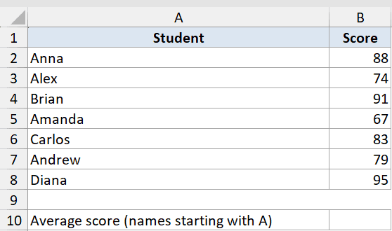
You want to find the average score for every student whose name starts with “A”.
Here is the formula:
=AVERAGEIF(A2:A8,"A*",B2:B8)
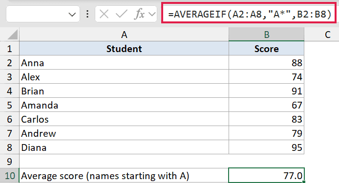
This returns 77. The * matches any text after A, so Anna (88), Alex (74), Amanda (67), and Andrew (79) are all included. Brian, Carlos, and Diana are skipped.
The ? wildcard works the same way but matches exactly one character. Use ? when you know the length of the match, and * when you just know the starting or ending text.
Example 4: Average Revenue for One Status
Here’s a real-world accounts scenario: averaging invoices that have a specific status.
The data has Invoice IDs in column A, Status in column B, and Revenue in column C, across rows 2 to 8. One row has a blank status.
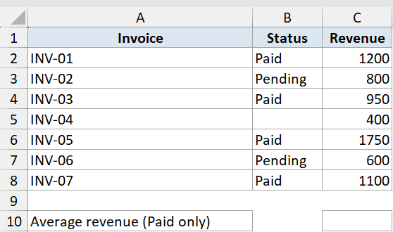
You want to find the average revenue for Paid invoices only.
Here is the formula:
=AVERAGEIF(B2:B8,"Paid",C2:C8)
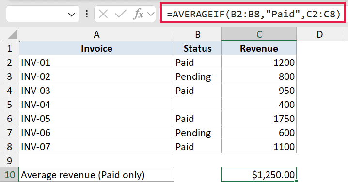
This returns 1250. Only INV-01 (1200), INV-03 (950), INV-05 (1750), and INV-07 (1100) are included. The blank-status row is ignored automatically because it does not match “Paid”.
To instead average everything except blank rows, use "<>" as the criteria. That tells AVERAGEIF to include only cells that are not empty.
Pro Tip: If no rows match your criteria, AVERAGEIF returns #DIV/0! Wrap it in IFERROR to show a fallback value instead: =IFERROR(AVERAGEIF(…),”No match”).
Example 5: Average Across Two Categories (AVERAGE + FILTER)
AVERAGEIF only accepts one criterion. When you need OR logic, AVERAGE combined with FILTER is the modern solution in Excel 365.
The data has Rep names in column A, Region in column B, and Q1 Sales in column C, across rows 2 to 8.
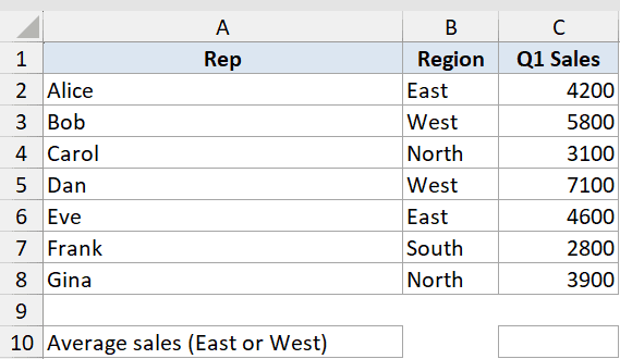
You want the average sales for reps in either East or West.
Here is the formula:
=AVERAGE(FILTER(C2:C8,(B2:B8="East")+(B2:B8="West")))
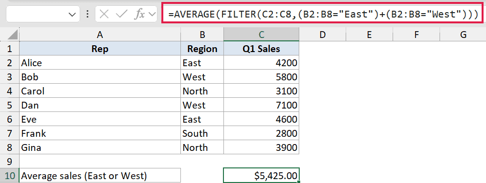
This returns 5425. FILTER uses + between the two conditions to act as OR, keeping any row where Region equals “East” or “West”. AVERAGE then calculates across those filtered rows only.
You cannot do this with AVERAGEIF alone. For AND logic across multiple conditions, use AVERAGEIFS instead.
Tips and Common Mistakes
- If AVERAGEIF returns #DIV/0!, no cells matched the criteria. Check for typos, extra spaces, or a mismatched range size. Wrap in IFERROR to handle it gracefully.
- Comparison operators like
>,<,>=,<>must be wrapped in quotes. Forgetting the quotes is the most common mistake. - AVERAGEIF is case-insensitive. “West”, “west”, and “WEST” all match the same rows.
- For two or more AND conditions, use AVERAGEIFS. For OR logic across multiple categories, use
=AVERAGE(FILTER(...))in Excel 365. - When average_range and range are different sizes, Excel anchors average_range to the top-left corner of your range argument. Always use the same dimensions to be safe.
AVERAGEIF is the go-to for a quick conditional average with one criterion. Start with the three-argument form for category averages, use the two-argument form when you check and average the same column, and reach for AVERAGE(FILTER(…)) whenever you need OR logic in Excel 365.
Related Excel Functions / Articles: