
If you want to pull everything after a character or phrase, the TEXTAFTER function gives you a direct way to do it.
In this article, I’ll show you how to use TEXTAFTER with positions, case matching, missing delimiters, and other practical options.
In Excel 365, you can also feed TEXTAFTER a range and the results will spill into the cells below.
TEXTAFTER Function Syntax in Excel
The TEXTAFTER function returns the text that appears after a delimiter you specify.
=TEXTAFTER(text, delimiter, [instance_num], [match_mode], [match_end], [if_not_found])
- text (required) is the text or cell reference you want to search.
- delimiter (required) is the character or text that marks where the returned text should begin.
- instance_num (optional) selects which occurrence of the delimiter to use. It defaults to 1, while a negative number counts from the end.
- match_mode (optional) controls case sensitivity. Use 0 for a case-sensitive match or 1 for a case-insensitive match. The default is 0.
- match_end (optional) treats the end of the text as a delimiter when set to 1. The default is 0.
- if_not_found (optional) supplies a custom result when Excel cannot find the delimiter. Otherwise, TEXTAFTER returns #N/A.
When to Use TEXTAFTER Function
- Extract a topic, code, label, or other value that follows a known delimiter.
- Return everything after the second, third, or another specific occurrence of a delimiter.
- Pull a file name or final segment from a path by counting delimiters from the end.
- Match delimiters without worrying about uppercase and lowercase letters.
- Replace #N/A with a helpful message when the delimiter is missing.
Example 1: Extract Text After a Delimiter
Let’s start with meeting entries that contain a room and a topic.
Below is the dataset. Column A contains each meeting entry, while columns B and C will extract the topic with two different formulas.
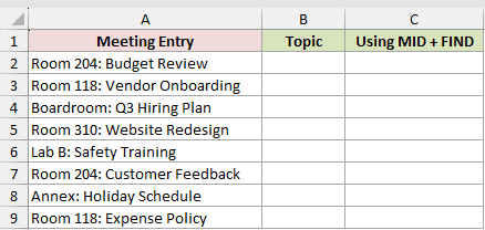
We want to return everything after the colon and space in each entry.
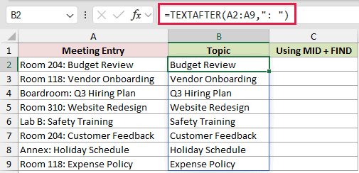
Here is the TEXTAFTER formula:
=TEXTAFTER(A2:A9,": ")
And here is the equivalent formula using MID, FIND, and LEN:
=MID(A2:A9,FIND(": ",A2:A9)+2,LEN(A2:A9))
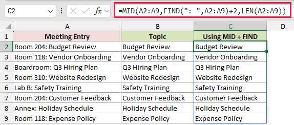
TEXTAFTER finds ": " in every entry and returns the text following it. The first result is Budget Review, and both formulas produce the same topics.
The MID version calculates where the delimiter ends, then returns the remaining characters. It works in older Excel versions, but TEXTAFTER is easier to read.
Pro Tip: Include the space in the delimiter when it should not appear in the result. Here, ": " removes both the colon and the following space.
Example 2: Return Text After the Nth Delimiter
Here’s how to work with text containing the same delimiter several times.
Below is the dataset. Column A contains cost center codes with four sections, and column B will return the final two sections.
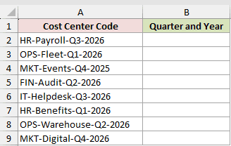
We want to return everything after the second hyphen in each code.
Here is the formula:
=TEXTAFTER(A2:A9,"-",2)
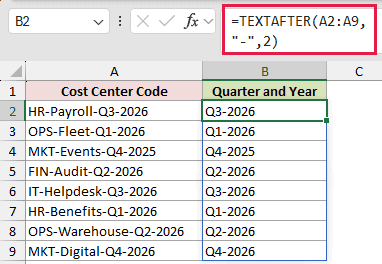
The instance_num argument is 2, so TEXTAFTER ignores the first hyphen and starts after the second one.
For example, the first code returns Q3-2026. The formula spills one result for each code in A2:A9.
Pro Tip: If instance_num is larger than the number of delimiters in the text, TEXTAFTER returns #N/A unless you supply if_not_found.
Example 3: Extract After the Last Delimiter
Now let’s count from the end of the text instead of the beginning.
Below is the dataset. Column A contains Windows file paths, while columns B and C will return the file name and its parent folder.
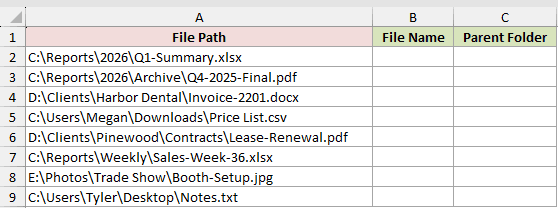
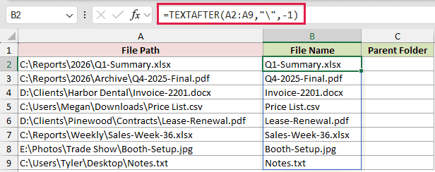
We first want to return the text after the final backslash in each path.
Here is the formula for the file name:
=TEXTAFTER(A2:A9,"\",-1)
We also want the folder immediately before each file name.
Here is the formula for the parent folder:
=TEXTAFTER(TEXTBEFORE(A2:A9,"\",-1),"\",-1)
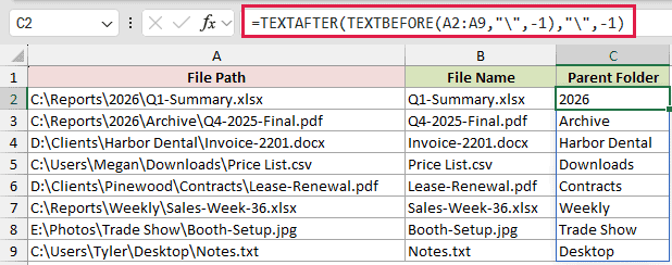
A negative instance_num counts delimiter occurrences from the right. Using -1 returns the text after the last backslash, such as Q1-Summary.xlsx.
For the parent folder, TEXTBEFORE removes the file name first. The outer TEXTAFTER then returns the final folder from the shortened path, such as 2026.
Example 4: Ignore Case When Matching a Delimiter
The delimiter in this example has inconsistent capitalization.
Below is the dataset. Column A contains shipping addresses using Apt, apt, or APT, while columns B and C compare two matching methods.
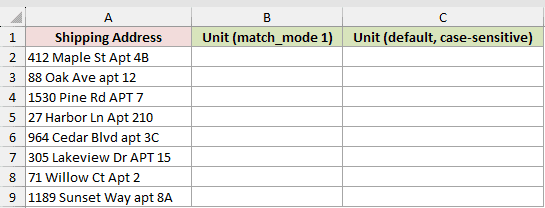
We want to extract every unit number regardless of how the word apt is capitalized.
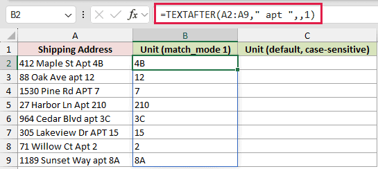
Here is the case-insensitive formula:
=TEXTAFTER(A2:A9," apt ",,1)
And here is the default case-sensitive formula for comparison:
=TEXTAFTER(A2:A9," apt ")
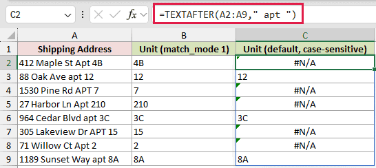
The two consecutive commas skip the optional instance_num argument. Setting match_mode to 1 lets the formula match Apt, apt, and APT.
The first result is 4B. The default formula matches only lowercase apt, so five of its eight results return #N/A.
Pro Tip: TEXTAFTER is case-sensitive by default. Use match_mode 1 when inconsistent capitalization should not affect the result.
Example 5: Treat the Text End as a Delimiter
Next, let’s handle rows where an optional note may be missing.
Below is the dataset. Column A contains delivery statuses, some followed by a location note, and column B will return that note.
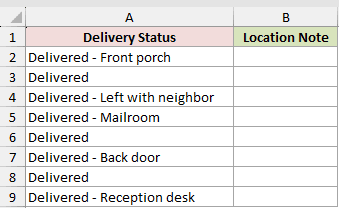
We want rows without a location note to return an empty string instead of #N/A.
Here is the formula:
=TEXTAFTER(A2:A9," - ",,,1)
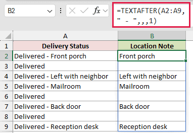
The three consecutive commas leave instance_num and match_mode at their defaults. The final 1 sets match_end to treat the text end as a delimiter.
Delivered – Front porch returns Front porch. A plain Delivered entry returns an empty string because no characters follow the virtual delimiter at the end.
Pro Tip: With the default first occurrence, match_end 1 returns an empty string when the delimiter is absent. Using -1 for instance_num would return the whole text instead.
Example 6: Return a Custom Value if Missing
Some help-desk notes do not include an escalation phrase.
Below is the dataset. Column A contains help-desk ticket notes, and column B will show the escalation team or a fallback message.
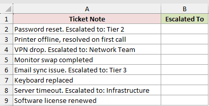
We want to return the team after Escalated to, or Not escalated when that phrase is missing.
Here is the formula:
=TEXTAFTER(A2:A9,"Escalated to: ",,,,"Not escalated")
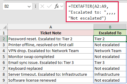
The fallback text goes in the sixth argument slot.
The first note returns Tier 2. The next note has no escalation phrase, so it returns Not escalated instead of #N/A.
This built-in argument is cleaner than wrapping the formula in IFERROR when you only need to handle a missing delimiter.
Tips & Common Mistakes
- TEXTAFTER is available in Excel for Microsoft 365 and Excel 2024. Earlier versions need an approach based on functions such as MID, FIND, SEARCH, and LEN.
- Matching is case-sensitive unless you set
match_modeto 1. Check capitalization when a delimiter appears present but the formula returns #N/A. - An
instance_numof 0 returns #VALUE!. Use a positive number to count from the beginning or a negative number to count from the end. - A missing delimiter returns #N/A unless
match_endorif_not_foundchanges that behavior. - A spilling formula needs empty cells in its output range. If another value blocks those cells, Excel returns #SPILL!.
- TEXTAFTER accepts more than one possible delimiter as an array constant, which helps when source text uses different separators.
- Use TEXTSPLIT when you need every segment from the text rather than only the portion after one delimiter.
TEXTAFTER handles many extraction jobs without the position calculations older formulas require.
Use a positive occurrence number to count from the start, or a negative one when the text you need is near the end.
Related Excel Functions / Articles:
