
Excel’s BITLSHIFT function moves the binary digits of a nonnegative whole number left and returns the resulting decimal value.
Each left shift adds a zero to the binary representation. A negative shift moves the bits right, which is useful when you need to discard lower bits.
In this article, I’ll show you how to build bit flags, pack RGB values, and turn IP addresses into sortable numbers.
BITLSHIFT Function Syntax in Excel
The BITLSHIFT function uses a number and a shift amount.
=BITLSHIFT(number, shift_amount)
- number is the nonnegative whole number whose bits you want to move.
- shift_amount controls how far the bits move. A positive value moves them left, while a negative value moves them right.
When to Use BITLSHIFT Function
- Create distinct flag values from bit positions.
- Convert quantities between binary storage units.
- Pack separate numeric fields into one value.
- Turn dotted IP addresses into numbers that sort correctly.
- Inspect how left and right shifts change binary digits.
Example 1: See How BITLSHIFT Moves Bits
Let’s begin by watching the bits move.
Below is the dataset. Columns A and B contain numbers and shift amounts, while columns C through E will hold the decimal and binary results.
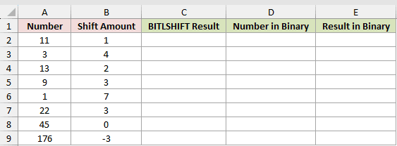
We want to shift every number by its corresponding amount with one formula.
Here is the BITLSHIFT formula:
=BITLSHIFT(A2:A9,B2:B9)
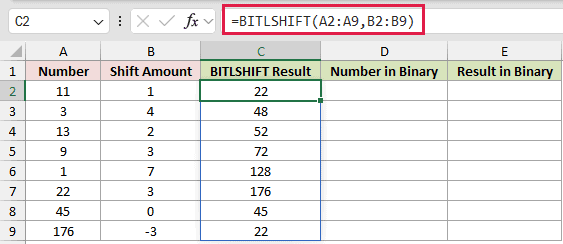
This range formula spills in Excel 2021, Excel 2024, and Microsoft 365. In Excel 2019 and earlier, enter a per-row version and fill it down.
The first row shifts 11 left by 1 and returns 22. A shift amount of 0 leaves 45 unchanged.
The last row shifts 176 by -3 and returns 22. That negative amount moves the bits right instead of returning an error.
Here is the formula that shows each original number in binary:
=BASE(A2:A9,2,8)
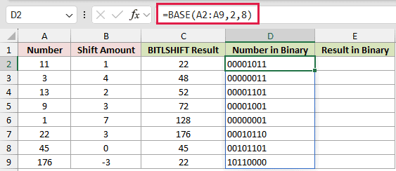
And here is the formula that shows each shifted result in binary:
=BASE(C2:C9,2,8)
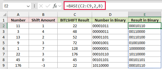
BASE displays 11 as 00001011. After the shift, 22 appears as 00010110, so you can see the zero added on the right.
Pro Tip: BASE works well for this view because it spills over a range. DEC2BIN returns one #VALUE! for a plain range and stops at 511.
Example 2: Build Flags From Bit Positions
Now let’s create a code for PPE issued to one worker.
Below is the dataset. It lists each PPE item, its bit position, and whether Marcus Reed received it. The flag column and code cell hold the results.
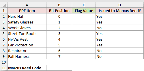
We want each bit position to produce its own flag value.
Here is the formula:
=BITLSHIFT(1,B2:B9)
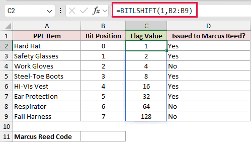
Positions start at 0. The resulting flags begin at 1, position 5 returns 32, and position 7 returns 128.
Next, we want to add the flags for the items marked Yes.
Here is the SUMIFS formula:
=SUMIFS(C2:C9,D2:D9,"Yes")
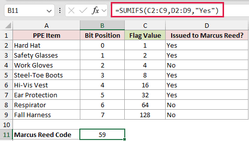
SUMIFS adds the selected flag values and returns Marcus Reed’s code of 59.
This setup keeps each item in its own bit. You can later test individual items without creating a separate column for every one.
Example 3: Convert Binary Storage Units
Here’s a practical way to convert file sizes into bytes.
Below is the dataset. The folder table contains sizes and units, while the lookup table maps each unit to a shift amount. Column D holds bytes.
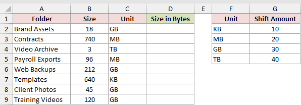
We want to choose the correct shift for each unit and return every size in bytes.
Here is the formula:
=BITLSHIFT(B2:B9,XLOOKUP(C2:C9,F2:F5,G2:G5))
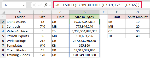
XLOOKUP returns the shift amount for each unit. BITLSHIFT then converts 18 GB to 19,327,352,832 bytes and 640 KB to 655,360 bytes.
XLOOKUP requires Excel 2021 or later.
These are binary units, where 1 KB equals 1,024 bytes. Each step from KB through TB adds 10 bits to the shift amount.
Pro Tip: This method is for binary units. If your source uses decimal storage units, use multiplication instead of BITLSHIFT.
Example 4: Pack RGB Values Into One Number
Next, we’ll combine separate color channels into one packed value.
Below is the dataset. Columns B through D contain red, green, and blue values. Columns E and F hold the packed number and hexadecimal check.
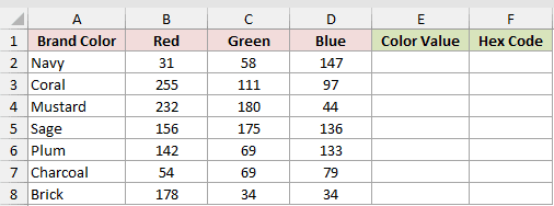
We want to move each channel into place and combine the channels into one number.
Here is the packing formula:
=BITLSHIFT(B2:B8,16)+BITLSHIFT(C2:C8,8)+D2:D8
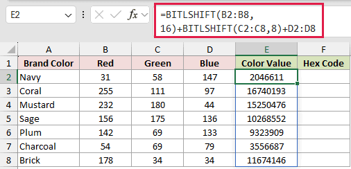
The formula shifts red by 16 bits and green by 8 bits, then adds blue. Navy returns a packed value of 2046611.
We can verify each packed value by displaying it as hexadecimal text.
Here is the BASE formula:
=BASE(E2:E8,16,6)
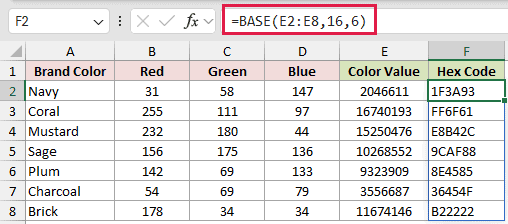
BASE converts Navy’s packed value to 1F3A93. Coral returns 16740193 and converts to FF6F61.
The matching hexadecimal text makes it easier to check that each channel landed in the intended position.
Example 5: Sort IP Addresses Numerically
Text sorting can put IP addresses in an order that looks wrong.
Below is the dataset. The left table contains devices and IP addresses. Column C holds numeric keys, and the table at the right holds the sorted results.
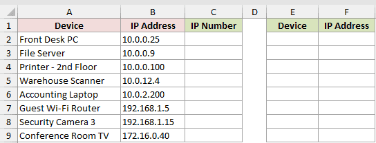
We first want to convert each dotted IP address into one sortable number.
Here is the formula entered in C2 and copied down:
=SUM(BITLSHIFT(--TEXTSPLIT(B2,"."),{24,16,8,0}))
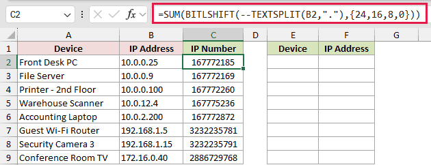
TEXTSPLIT separates the address. BITLSHIFT moves each part into position, and SUM collapses the shifted parts into one number for that row.
The double unary makes the text-to-number conversion explicit. Testing showed BITLSHIFT also converted the split text without it, so it isn’t required.
The File Server address becomes 167772169. The Front Desk PC becomes 167772185, and the Printer address becomes 167772260.
Now we can sort the original device and address columns by those numeric keys.
Here is the SORTBY formula:
=SORTBY(A2:B9,C2:C9)
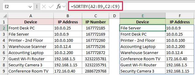
The sorted list starts with 10.0.0.9, followed by 10.0.0.25 and 10.0.0.100. A text sort would place 10.0.0.100 before 10.0.0.9.
This setup needs Excel 2024 or Microsoft 365 because it uses TEXTSPLIT. SORTBY itself is available in Excel 2021 and later.
Example 6: Troubleshoot BITLSHIFT Errors
Finally, let’s test the inputs that often cause confusion.
Below is the dataset. Columns A and B contain the Number and Shift Amount inputs. Column C, headed “BITLSHIFT Result,” will hold the results.
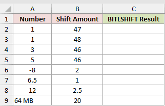
We want one spill to show which combinations work and which fail.
Here is the formula:
=BITLSHIFT(A2:A9,B2:B9)
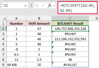
The error cells are intentional. Each row isolates a different rule:
- BITLSHIFT accepts a number only up to
2^48-1(281,474,976,710,655), and the result must stay within the same limit. Shifting 1 by 47 works and returns 140,737,488,355,328, while shifting 1 by 48 deliberately returns#NUM!. - Shifting 3 by 46 works and returns 211,106,232,532,992. Shifting 5 by 46 deliberately returns #NUM! because its result would be too large.
- The -8 row deliberately returns #NUM! because the number itself cannot be negative.
- The 6.5 row deliberately returns #NUM! because BITLSHIFT requires a whole number.
- The 2.5 shift is silently truncated toward zero, so 12 shifted by 2.5 returns 48.
- The “64 MB” row deliberately returns #VALUE! because the text is not a numeric value.
Pro Tip: A decimal shift does not trigger an error. Excel truncates it toward zero, which can hide a data-entry mistake.
Tips & Common Mistakes
- BITLSHIFT is available in Excel 2013 and later. Range formulas spill only in versions that support dynamic arrays.
- A negative shift moves bits right and discards bits that fall off the end. Shifting 5,500,000 right by 20 returns 5.
- Numbers stored as text can convert automatically, but text containing labels or units returns #VALUE!.
- BITOR can combine flag values when they might overlap. Plain addition is safe only when every flag occupies a different bit.
- BITRSHIFT is the clearer choice when unpacking fields. For Navy’s packed value 2046611, BITRSHIFT with BITAND retrieves 31, 58, and 147.
- Keep result size in mind. A valid input can still return
#NUM!when a left shift makes the result too large.
Use BITLSHIFT when building flags or packing numeric fields into fixed bit positions.
Keep the result limit and silent shift truncation in mind, especially when shift amounts come from worksheet cells.
Related Excel Functions / Articles:
