
A running count of occurrences numbers each repeat of a value as you go down a list.
The first Billing ticket gets 1, the next one gets 2, and so on.
Excel doesn’t have a button for this.
You do it with a range that starts at a fixed first row and stops at the current row, so it grows by one row at a time.
That growing range is also where things go wrong. Lock both ends and you get a total count.
Put the formula in an Excel Table and it can quietly break when you add a row.
In this article, I’ll show you six ways to get a running count, using COUNTIF, COUNTIFS, a single MAP formula, a Table-safe formula, and a case-sensitive version.
I’ll also cover some practical uses, like “2 of 4” labels.
Method #1: Using the COUNTIF Function
COUNTIF with a growing range is the classic way to do a running count, and it works in every version of Excel.
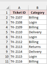
Below I have a dataset on the Ticket Log sheet with ticket IDs in column A and their categories in column B.
I want column C to show which occurrence of its category each ticket is.
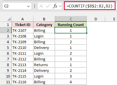
Here is the formula I entered in C2 and then filled down to C11:
=COUNTIF($B$2:B2,B2)
How does this formula work?
The range $B$2:B2 starts at B2, which is locked with dollar signs. The end, B2, has no dollar signs, so it moves down as you fill the formula.
In C4, the range becomes $B$2:B4. COUNTIF counts how many times “Billing” appears in B2:B4, which is 2. So TK-2109 is the second Billing ticket.
By C11, the range covers the whole list, and TK-2116 shows 4 because it’s the fourth Billing ticket.
Note: When you type the formula, click on B2 and press F4 once to turn it into $B$2. Keep the second B2 as it is.
Method #2: Using COUNTIF With IF (One Specific Value)
Sometimes you only care about one value. For example, you may want to number the Billing tickets and leave every other row blank.
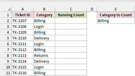
Below I have the same ticket list on the One Category sheet.
The category I want to count, Billing, is in cell E2. That way I can change it later without touching the formula.
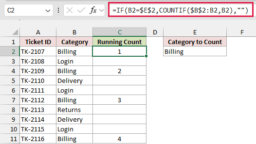
Here is the formula I entered in C2 and filled down to C11:
=IF(B2=$E$2,COUNTIF($B$2:B2,B2),"")
How does this formula work?
The IF part checks whether the category in column B matches the one in E2. The $E$2 reference is locked so every row looks at the same cell.
When it matches, the formula runs the same COUNTIF from Method #1. When it doesn’t, it returns an empty string, so the cell looks blank.
The four Billing tickets get 1, 2, 3, and 4. If you change E2 to Login, the column recounts for Login tickets instead.
Method #3: Using the COUNTIFS Function
Here’s the same idea when two columns together decide what counts as a repeat.
Below I have a dataset on the Customer Issues sheet with case IDs in column A, customer names in column B, and issue types in column C.
I want a running count for each customer and issue pair.
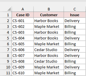
Here is the formula I entered in D2 and filled down to D11:
=COUNTIFS($B$2:B2,B2,$C$2:C2,C2)
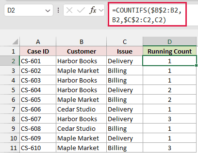
How does this formula work?
COUNTIFS only counts a row when every condition is true. The first growing range checks the customer, and the second checks the issue.
So a Billing case for Harbor Books doesn’t bump its Delivery count.
CS-604 is the second Harbor Books Delivery case, so D5 shows 2. CS-607 is the third, so D8 shows 3.
Both growing ranges have to cover the same rows. If one ends on a different row, the ranges are different sizes and COUNTIFS returns a #VALUE! error.
Method #4: Using the MAP Function (Microsoft 365)
If you have Microsoft 365, you can get the whole running count from one formula that spills down the column. There’s nothing to fill down.
Below I have the same ticket list (on the MAP Formula sheet), with ticket IDs in column A and categories in column B.
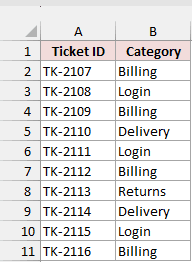
Here is the formula I entered in C2:
=MAP(B2:B11,LAMBDA(x,COUNTIF(B2:x,x)))
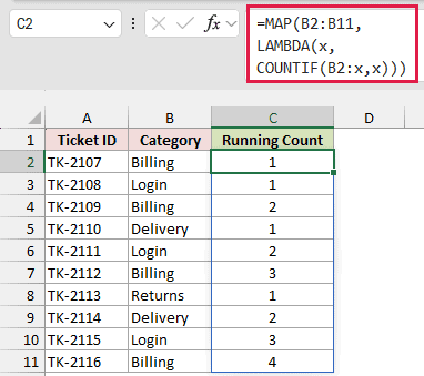
How does this formula work?
MAP goes through B2:B11 one cell at a time and hands each cell to the LAMBDA as x.
B2:x then builds a range from B2 down to that cell. That’s the same growing range as $B$2:B2 in Method #1, just built inside one formula.
COUNTIF counts x in that range, and MAP returns all ten results at once. You get 1, 1, 2, 1, 2, 3, 1, 2, 3, 4, exactly like Method #1.
Note: MAP and LAMBDA are available in Microsoft 365 and Excel 2024. In older versions, use the COUNTIF formula from Method #1.
Method #5: Using COUNTIF With Structured References (Excel Tables)
If your data is in an Excel Table, the formula from Method #1 can give you wrong numbers once you start adding rows.
Below I have the ticket list converted into an Excel Table on the Ticket Table sheet (select any cell in the data and press Ctrl + T to do this).
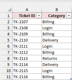
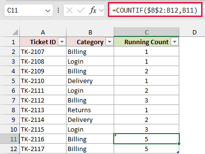
Here’s the problem. I used =COUNTIF($B$2:B2,B2) in the Table, then typed a new ticket, TK-2117 (Billing), in the row right below it.
The Table grew to include the new row, but Excel also changed the formula in C11 to =COUNTIF($B$2:B12,B11). Now TK-2116 shows 5 when it should show 4.
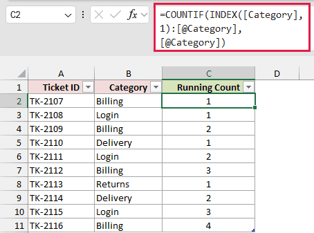
Here is the formula that doesn’t break. I entered it in C2, and the Table filled it down the whole column on its own:
=COUNTIF(INDEX([Category],1):[@Category],[@Category])
How does this formula work?
INDEX([Category],1) returns the first cell of the Category column. [@Category] is the Category cell in the current row.
Put a colon between them and you get a range from the first row down to the current row.
That’s the growing range again, but this time both ends are Table references.
Excel doesn’t rewrite Table references when the Table grows, so every row keeps counting the right range.
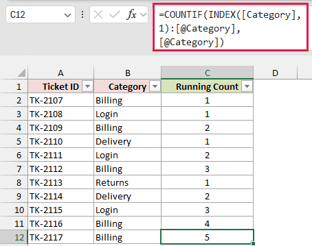
Now when I type TK-2117 (Billing) below the Table, TK-2116 still shows 4 and the new row shows 5.
Method #6: Using SUMPRODUCT and EXACT (Case-Sensitive)
COUNTIF and COUNTIFS ignore letter case, so “SAVE10” and “save10” count as the same thing. When case matters, like with coupon codes, you need a different formula.
Below I have a dataset on the Coupon Codes sheet with order IDs in column A and the coupon code used in column B.
Some codes differ only in upper and lower case.
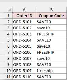
Here is the formula I entered in C2 and filled down to C11:
=SUMPRODUCT(--EXACT($B$2:B2,B2))
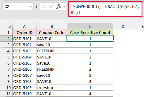
How does this formula work?
EXACT compares each code in the growing range with the current code and returns TRUE only for an exact match, including case.
The double minus turns those TRUE and FALSE values into 1s and 0s, and SUMPRODUCT adds them up. It works in every version of Excel.
To see the difference, I put the regular COUNTIF formula next to it in column D.
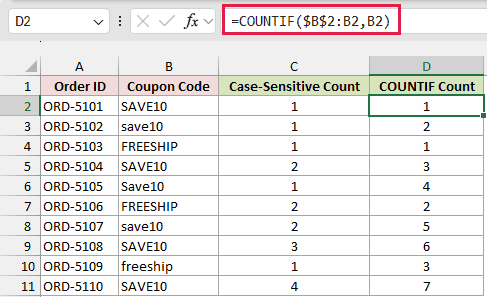
The EXACT version counts SAVE10 as 1, 2, 3, 4. COUNTIF lumps SAVE10, save10, and Save10 together, so ORD-5110 shows 7 instead of 4.
Practical Uses of a Running Count in Excel
A running count is handy on its own, but it’s even more useful as a building block. Here are a few examples, all using the ticket list.
Running Count vs Total Count
A running count and a total count use almost the same formula, and people often mix them up.
Below I have the ticket list on the Running vs Total sheet, with the running count from Method #1 already in column C.
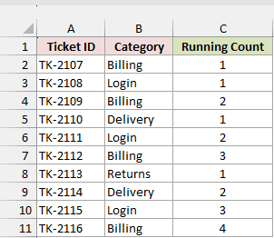
Here is the total count formula I entered in D2 and filled down to D11:
=COUNTIF($B$2:$B$11,B2)
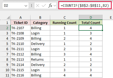
The only change is the extra dollar signs in $B$11. The range no longer grows, so every Billing row shows 4, the total number of Billing tickets.
Use the running count when you need the order of each repeat, and the total count when you need how many times a value shows up overall.
Labeling Each Row as “2 of 4”
With both counts side by side, you can label each row with its place in the group.
On the same sheet, with the running count in column C and the total count in column D, I entered this formula in E2 and filled it down:
=C2&" of "&D2
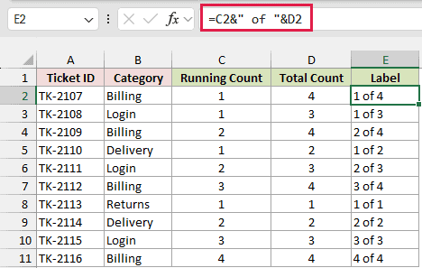
The ampersand joins the two numbers with the text ” of “. TK-2109 gets “2 of 4” because it’s the second of four Billing tickets.
Creating Lookup Keys for the Nth Occurrence
A regular lookup only finds the first match. If you want the second Billing ticket, you need a key that’s unique for every occurrence.
On the same sheet, I entered this formula in F2 and filled it down:
=B2&"-"&C2
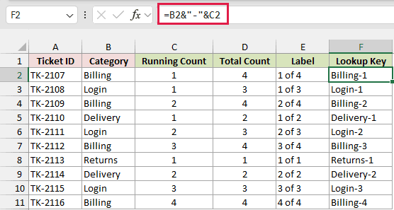
This joins the category and its running count, so the Billing tickets become Billing-1, Billing-2, Billing-3, and Billing-4.
Now I can look up any occurrence. I typed Billing-2 in H2 and used this formula in I2:
=XLOOKUP(H2,F2:F11,A2:A11)
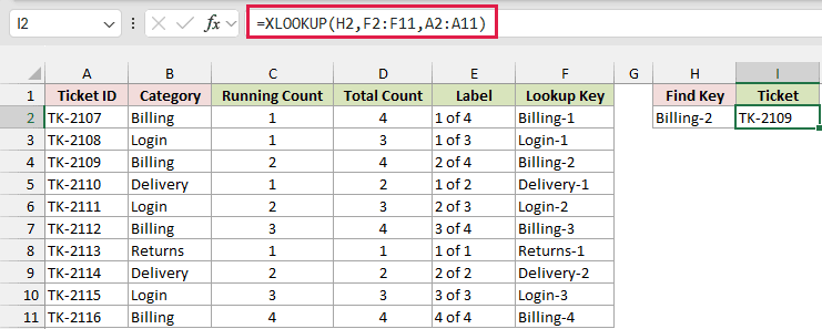
It returns TK-2109, the second Billing ticket. XLOOKUP needs Excel 2021 or later. In older versions, =INDEX(A2:A11,MATCH(H2,F2:F11,0)) does the same job.
Keeping Only the First N Occurrences
You can also use the running count to keep just the first few tickets of each category.
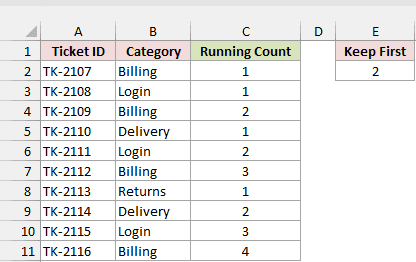
Below I have the ticket list on the First N sheet with the running count in column C.
The number of tickets to keep per category, 2, is in cell E2.
Here is the formula I entered in G2:
=FILTER(A2:B11,C2:C11<=E2)
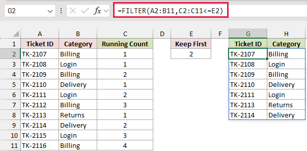
FILTER keeps every row whose running count is 2 or less. It returns seven tickets: the first two Billing, Login, and Delivery tickets, plus the only Returns ticket.
FILTER needs Excel 2021 or later. In older versions, turn on a filter for the Running Count column and show only values less than or equal to 2.
Additional Notes About Running Counts in Excel
- A running count depends on row order. If you sort the data, the counts recalculate for the new order.
- Keep the first cell of the range absolute and the last cell relative. If both are locked, you get a total count instead.
- Extra spaces make two values look the same when they aren’t. If a count looks split, clean up the source data first.
- COUNTIF and COUNTIFS treat
*and?as wildcards (and~as an escape character). So a value like “A*” also counts “AB”. The EXACT formula from Method #6 doesn’t have this problem. - Each row counts from the top of the list again, so very long lists can recalculate slowly. The formulas still work; they just take longer.
Frequently Asked Questions
Here are answers to a few common questions about running counts in Excel.
How do I get Excel to count 1, 2, 3 down a column?
If you just want sequential numbers, use =SEQUENCE(10) in Excel 2021 or Microsoft 365, or =ROW()-1 filled down from row 2.
A running count is different. It starts again at 1 for each new value.
Can the first occurrence show zero instead of one?
Yes. Subtract 1 from any of the formulas, for example =COUNTIF($B$2:B2,B2)-1. The first occurrence then shows 0 and the second shows 1.
Why does every row of a value show the same number?
The end of your range is probably locked, like $B$2:$B$11. That gives you the total count. Remove the dollar signs from the second cell so the range can grow.
Will new rows get a running count automatically?
In a normal range, copy the formula down to the new rows.
In an Excel Table, the formula fills in on its own. Use the Table version from Method #5 so the counts stay correct.
Conclusion
In this article, I showed you six ways to calculate a running count of occurrences in Excel, from a simple COUNTIF formula to a case-sensitive version.
Every one of them uses the same idea, a range that starts at a fixed row and grows by one row at a time.
For most lists, I’d go with COUNTIF.
I hope you found this article helpful.
Other Excel articles you may also like:
