
A running total in Excel shows you the total so far on every row. It’s also called a cumulative sum.
A running balance carries forward an opening balance, adding money in and subtracting money out. I’ll show you formulas, an Excel Table, a PivotTable, and Power Query.
Here’s a quick comparison to help you pick the approach that fits your list.
| Method | Works in | Pick it when |
|---|---|---|
| SUM | Every Excel version | You want the usual running total |
| Adding the previous total | Every Excel version | You want a simple carry-forward calculation |
| SCAN | Microsoft 365, web, Excel 2024 | You want one formula for every row |
| SUM and INDEX | Excel 2010 and later | You regularly add new receipts |
| SUMIF | Every Excel version | You need separate totals by market |
| SUBTOTAL | Every Excel version | You want totals for visible rows |
| PivotTable | Every Excel version | You need a daily summary |
| Power Query | Excel 2016 and later | You already import or clean data |
Method #1: Using the SUM Function
I recommend SUM for most people. It works in every Excel version, and you only need to understand one expanding range.
Below I have a dataset of daily farmers market receipts, with Receipt ID, Date, Market, and Amount in columns A:D on the Cumulative Sum sheet.
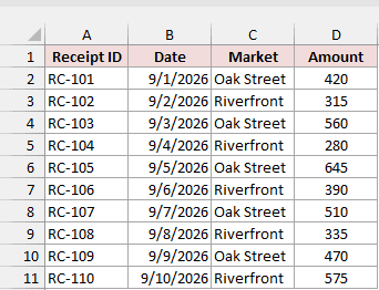
You want a running total beside each receipt, starting with 420 and ending with 4,500.
Type SUM Total in E1. Enter the formula below in E2, then copy it down to E11.
To copy it, double-click the fill handle, the small square at E2’s bottom-right corner, or drag it down to E11.
=SUM($D$2:D2)
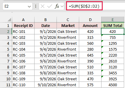
How does this formula work?
The dollar signs lock the first cell, $D$2, so it stays at D2 when you copy the formula.
The ending cell, D2, stays unlocked and moves down one row with each copy. That makes the range grow each time.
The formula becomes =SUM($D$2:D3) in E3 and =SUM($D$2:D11) in E11.
SUM adds everything from the first receipt through the current row.
Each row has its own copy of the formula.
Running Balance With an Opening Balance
For a cash ledger, you can use the same expanding ranges to add receipts and subtract expenses from an opening balance.
Below I have Transaction ID, Date, Description, Money In, and Money Out in A:E on the Running Balance sheet, plus an opening balance of 1,000 in B13.
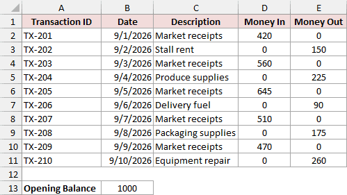
You want the balance after each transaction. Enter money in and money out as positive amounts, using zero in the unused column.
Type SUM Balance in F1. Enter this formula in F2, then double-click the fill handle or drag it down to F11.
=$B$13+SUM($D$2:D2)-SUM($E$2:E2)
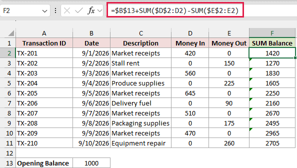
The formula starts with the locked opening balance in B13, adds all money in so far, and subtracts all money out so far.
You’ll see 1,420 after the first receipt and 1,270 after paying stall rent. The final running balance is 2,705 in F11.
Method #2: Adding the Previous Total
Here’s another way to calculate it. Instead of adding an expanding range, you can carry the previous total forward.
Below I have daily farmers market receipts on the Cumulative Sum sheet, with Receipt ID, Date, Market, and Amount in columns A:D.
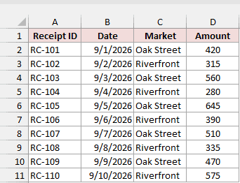
You want to add each receipt to the total immediately above it. Type Add Previous in E1.
Here’s how to set it up in two steps.
- Enter the following formula in E2. The first total is just the first receipt amount.
=D2
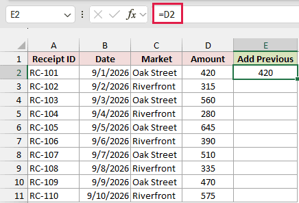
- Enter the following formula in E3, then double-click the fill handle or drag it down to E11.
=E2+D3
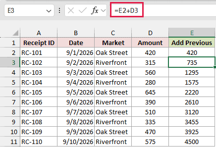
The formula adds 315 from D3 to the previous total of 420 in E2, returning 735. Each row repeats that carry-forward calculation.
You’ll finish with 4,500 in E11, matching the SUM method.
Note: If you delete a row in the middle, the formula below it loses its preceding-cell reference. That produces #REF! there and in every total below. I recommend Method #1 as the safer default because its SUM ranges recalculate after deletion.
Method #3: Using the SCAN Function
If you’d prefer to enter one formula, you can use SCAN to return every running total at once.
SCAN works in Microsoft 365, Excel for the web, and Excel 2024. It isn’t available in Excel 2021 or older.
Below I have daily farmers market receipts on the Cumulative Sum sheet, with Receipt ID, Date, Market, and Amount in A:D.
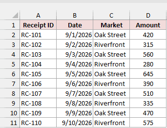
You want one cumulative sum for each amount in D2:D11, without copying a formula down.
LAMBDA lets you define a small calculation for SCAN to repeat. It names the calculation’s inputs and describes what to do with them.
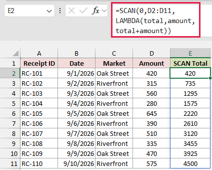
Type SCAN Total in E1 and enter this formula in E2. Keep E3:E11 empty so your results can spill down automatically.
=SCAN(0,D2:D11,LAMBDA(total,amount,total+amount))
How does this formula work?
SCAN starts at zero and works through D2:D11 in order. At each row, it adds the current amount to the accumulated total.
Here, total and amount are names chosen for LAMBDA’s two inputs. The total input is the accumulated value, and amount is the current receipt.
SCAN returns each intermediate total, rather than only the final sum. You’ll see 420 in E2, 735 in E3, and 4,500 in E11.
Running Balance With SCAN
For a running balance, you can start SCAN with an opening balance and add each transaction’s net change.
Below I have Transaction ID, Date, Description, Money In, and Money Out in A:E on the Running Balance sheet, plus an opening balance of 1,000 in B13.
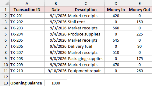
You want the balance after every receipt or expense. Type SCAN Balance in F1 and enter this formula in F2, leaving F3:F11 empty.
=SCAN($B$13,D2:D11-E2:E11,LAMBDA(total,amount,total+amount))
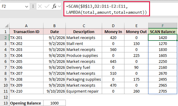
SCAN starts with 1,000 from B13 instead of zero. The D2:D11-E2:E11 part subtracts each row’s money out from its money in.
SCAN adds those net changes to the balance, returning 1,420 after the first transaction and 2,705 after the last.
Note: These source ranges are fixed and end at row 11. Extend them when you add transactions below that row. Enter SCAN outside an Excel Table because spilled formulas return #SPILL! inside a Table.
Method #4: Using SUM and INDEX (Excel Tables)
If you regularly add receipts, you can use an Excel Table to extend the running-total formula into new rows automatically.
Below I have daily farmers market receipts on the Table Receipts sheet, with Receipt ID, Date, Market, and Amount in A:D.
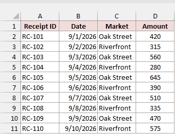
You want a running total that stays correct as your receipt list grows. Start by turning this range into a Table and adding a formula column.
Here’s how to set it up.
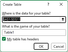
- Select any cell in the data and press Control + T (Command + T on a Mac). Make sure My table has headers is checked, then click OK.
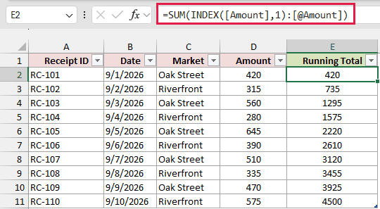
- Type Running Total in E1 to expand the Table. Enter the following formula in E2. Excel fills the whole column automatically.
=SUM(INDEX([Amount],1):[@Amount])
How does this formula work?
The INDEX([Amount],1) part refers to the first Amount cell. The [@Amount] part refers to the Amount in the current row.
The colon joins those endpoints into a range. SUM adds that range, finishing at 4,500 in E11.
This gives each Table row its own formula, called a calculated column. Type new receipts directly below the Table, and Excel adds the formula automatically.
Inside a Table, an ordinary =SUM($D$2:D2) can go wrong as the Table grows. Excel adjusts the old last row’s reference, making its range jump ahead.
If I use =SUM($D$2:D2) inside the Table and add receipt RC-111 for 200 directly below it, RC-110’s formula changes to =SUM($D$2:D12).
That makes RC-110 show 4,700 instead of 4,500.
The INDEX version stays correct because it always starts at the first Amount cell and ends at the current row’s Amount.
Method #5: Using the SUMIF Function
If you need a separate running total for each market, you can use SUMIF to add only matching receipts.
Below I have daily farmers market receipts on the By Market sheet, with Receipt ID, Date, Market, and Amount in columns A:D.
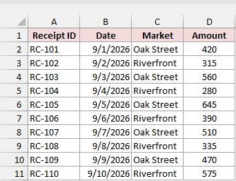
You want separate cumulative sums for Oak Street and Riverfront, even though the rows alternate between those markets.
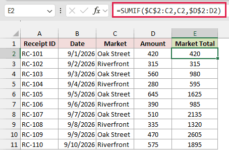
Type Market Total in E1. Enter this formula in E2, then double-click the fill handle or drag it down to E11.
=SUMIF($C$2:C2,C2,$D$2:D2)
How does this formula work?
SUMIF checks the markets from the first row through the current row with $C$2:C2. The C2 part is the market to match.
SUMIF adds the corresponding amounts in $D$2:D2 only when their market matches. Both ranges expand together as you copy down.
You’ll see 420 for Oak Street’s first receipt and 315 for Riverfront’s first receipt. Oak Street’s next total is 980, adding 420 and 560.
The final totals are 2,605 for Oak Street in E10 and 1,895 for Riverfront in E11. Each market has its own running total.
Method #6: Using the SUBTOTAL Function
If you want your running total to change when you filter the list, you can use SUBTOTAL.
Below I have a filterable Table of daily farmers market receipts on the By Market sheet, with Receipt ID, Date, Market, and Amount in A:D.
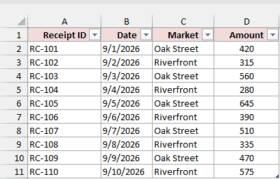
You want to total only the visible receipts through each row, so you can filter for a market and see its running total.
Type Visible Total in E1. Enter this formula in E2, then double-click the fill handle or drag it down to E11.
=SUBTOTAL(109,$D$2:D2)
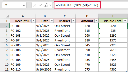
With all rows visible, you’ll see the usual running totals, ending at 4,500 in E11.
The 109 setting sums the expanding range while ignoring filtered rows and manually hidden rows. The 9 setting ignores filtered rows but includes manually hidden rows.
Now filter the list to show Oak Street receipts.
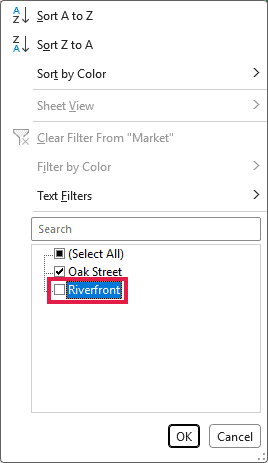
- Click the filter arrow in the Market header. Uncheck Riverfront so only Oak Street is checked, then click OK.
You’ll now see only Oak Street’s receipts. The visible running totals are 420, 980, 1,625, 2,135, and 2,605.
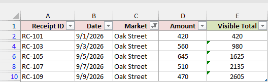
The last visible row shows 2,605. Clear the Market filter to bring back all receipts and the full total of 4,500.
Method #7: Creating a PivotTable
If you want a daily summary rather than a total beside each receipt, you can create a PivotTable.
A PivotTable groups receipts by date and adds their amounts. From there, you can show a running total beside each daily amount.
Below I have daily farmers market receipts in A1:D11 on the Cumulative Sum sheet, with Receipt ID, Date, Market, and Amount.
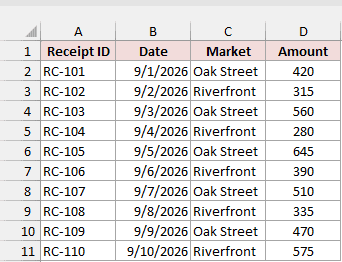
You want a daily amount and a cumulative amount for each date. Follow these steps to build the summary on a separate sheet.
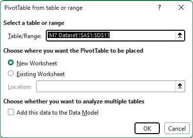
- Select any cell in the receipts data. Go to Insert > PivotTable, keep New Worksheet selected, and click OK.
- In the PivotTable Fields pane, drag Date to Rows and Amount to Values. If you see Sep instead of individual dates, right-click a date in the PivotTable and choose Ungroup.
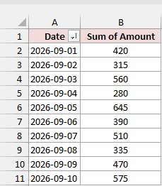
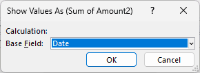
- Drag Amount into Values a second time. Right-click any number in this second column, choose Show Values As, then choose Running Total In.
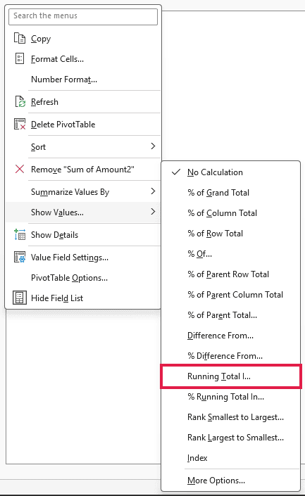
- Choose Date as the Base field in the dialog, then click OK.
- Click the value headers and rename them Daily Amount and Running Total. Go to Design > Grand Totals > Off for Rows and Columns. You can name the sheet Daily Summary.
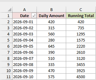
The PivotTable shows one row per date, with running totals from 420 through 4,500. It adds multiple receipts on the same date into that day’s amount.
Keep Date, your base field, in oldest-to-newest order so the running total follows the dates.
The PivotTable doesn’t update on its own. After changing the source data, right-click the PivotTable and choose Refresh.
You can choose % Running Total In from the same menu if you want each cumulative amount as a percentage of the grand total.
Method #8: Using Power Query
If you already import or clean receipts in Power Query, you can add a running-total column as part of that preparation.
Power Query is Excel’s built-in tool for importing and cleaning data. It loads the result as a new Table, keeping your original receipts in their source Table.
You need an Excel Table first. Select the receipts, press Control + T (Command + T on a Mac), confirm the headers, and name the Table QueryReceipts using Table Design > Table Name.
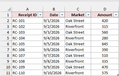
Below I have a Table named QueryReceipts on the Query Source sheet, containing Receipt ID, Date, Market, and Amount for the daily farmers market receipts.
You want a running total in the query result, ending at 4,500. Follow these steps to sort the receipts and calculate it.
- Select a cell in QueryReceipts and go to Data > From Table/Range. The Power Query Editor opens with your receipts.
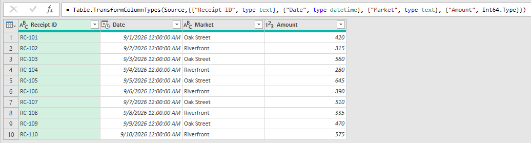
- Click the Date column filter arrow and choose Sort Ascending. Then click the Receipt ID arrow and choose Sort Ascending. Receipt ID breaks ties between receipts on the same date.
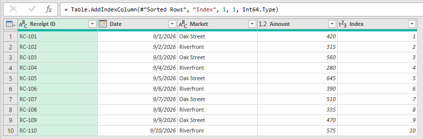
- Go to Add Column > Index Column > From 1. This adds an Index column numbered 1 through 10.
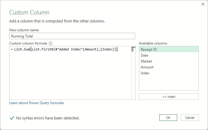
- Go to Add Column > Custom Column. Name the column Running Total, enter the following formula in the formula box, and click OK.
List.Sum(List.FirstN(#"Added Index"[Amount],[Index]))
How does this formula work?
The #"Added Index" reference names the previous step, created when you added the index. The [Amount] part returns that step’s entire Amount column as a list.
The [Index] value tells List.FirstN how many amounts to keep. For row 3, for example, it keeps the first three receipt amounts.
The List.Sum function adds those amounts, returning the cumulative sum for that row. Use your actual index step’s name if it differs in Applied Steps.
- Go to Home > Close & Load. Excel loads the result as a new Table on a new sheet, which you can name Query Result.
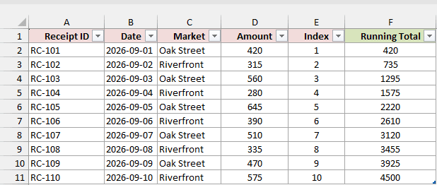
The result Table has the receipt columns plus Index and Running Total. Its last row shows 4,500.
After changing the source receipts, use Data > Refresh All. The query doesn’t refresh its results automatically when you edit the source Table.
The query re-adds all the earlier amounts for every row. That’s fine for a few thousand rows, but calculations slow down with very large datasets.
Additional Notes About Running Totals in Excel
Before you rely on the totals, check these details in your source data.
- Sort complete records by date first. A running total follows row order, which may differ from date order in an unsorted list.
- Numbers stored as text need converting to real numbers. SUM silently skips them, while the plus sign in Method #2 converts them during addition.
- Text like “n/a” in Amount is ignored by SUM. The previous-total formula and SCAN return #VALUE! from that row down, so check for these entries.
- Blank amount cells count as zero in every formula method shown here. Leave an amount blank when you mean zero.
- Deleted rows can break Method #2. The SUM, SCAN, and Table methods recalculate after you insert or delete rows.
Frequently Asked Questions
Here are a few questions that come up a lot with running totals.
How do I calculate a running total across columns instead of rows?
For a running total across row 2, keep the starting cell fixed and move the endpoint. For amounts starting in B2, enter this in another row and copy right.
=SUM($B$2:B2)
Column B stays locked while the ending column changes with each copy.
How do I convert running totals to fixed values?
Copy the running-total column, then use Paste Special > Values to replace its formulas with the current results.
With SCAN, copy the entire spill range and paste it as values.
Can a running balance go below zero?
Yes, the formulas return a negative balance when your money out exceeds your available balance. You can use Conditional Formatting to highlight negative amounts.
How do I chart a running total?
Select the date column and running-total column, then go to Insert and choose a Line chart.
The line rises when every amount is positive because each receipt increases the total so far.
Conclusion
I’ve shown you how to calculate running totals with formulas, an Excel Table, a PivotTable, and Power Query, plus running balances.
For most worksheets, I recommend starting with SUM because it’s simple and easy to follow.
I hope you found this article helpful.
Other Excel articles you may also like:
