
You have an Excel formula such as =Denver!C10, but it keeps pointing to Denver when you need another sheet.
You’d rather type a sheet name in a cell and have the formula follow your choice.
I’ll show you how to pull a store total, then match individual items. I’ll also cover an alternative for a fixed list of sheets.
Method #1: Using the INDIRECT Function
I recommend this approach for most people because you can type any sheet name without changing the formula.
INDIRECT turns text into a real cell reference.
Below I have a dataset of outdoor-gear sales on three store sheets named Denver, Boise and Salt Lake City, all with the same layout.
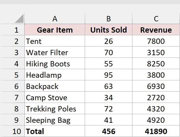
I keep total revenue in C10 on each sheet. You can see the Salt Lake City sheet below, with gear items and their sales in A1:C10.
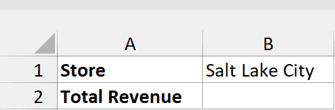
On the INDIRECT sheet, I have Store in A1 and Salt Lake City in B1. You can type a different sheet name in B1.
Total Revenue is in A2, with B2 empty before entering the formula.
You can enter this formula in B2 to pull total revenue from the sheet named in B1.
=INDIRECT("'"&B1&"'!C10")
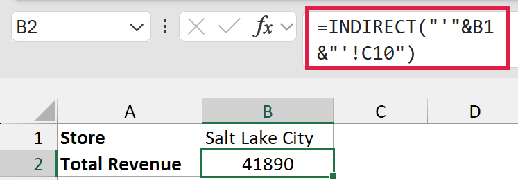
You get 41890 in B2, the total revenue from Salt Lake City’s C10. You can also see the formula in the formula bar.
How does this formula work?
B1 contains the sheet name Salt Lake City.
The expression "'"&B1&"'!C10" builds the text 'Salt Lake City'!C10. The & characters join the sheet name to the rest of the reference.
INDIRECT turns that text into a real reference and returns the value from C10 on that sheet.
Now you can change B1 to Boise, and the total updates on its own.
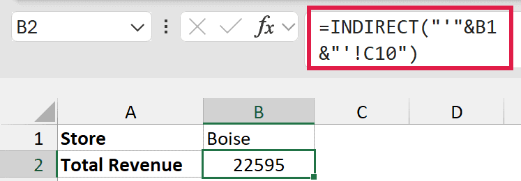
You get 22595 for Boise. If you enter Denver instead, you get 33645.
Note: Single quotes are needed around Salt Lake City because the name contains spaces. Keeping them for names without spaces works too.
Method #2: Using INDIRECT and XLOOKUP
When you need each item’s revenue, you can use XLOOKUP to find it by name, even when the items appear in a different order.
You can use this version in Microsoft 365, Excel 2021 and later.
Below I have a dataset of outdoor-gear sales on the Denver, Boise and Salt Lake City sheets. Each store lists the same items in a different order.
You can see the Boise sheet below. I have gear items in A2:A9 and revenue in C2:C9, with totals in row 10.
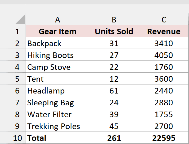
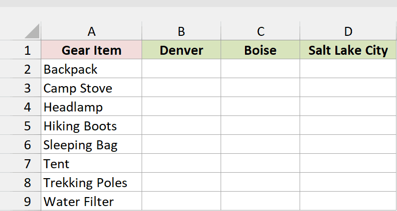
On the INDIRECT and XLOOKUP sheet, I list the gear items alphabetically in A2:A9, under Gear Item in A1.
I put the store names Denver, Boise and Salt Lake City in B1:D1. You use those headers as the sheet names for the formulas.
B2:D9 starts empty, ready for each store’s revenue figures.
You can enter this formula in B2.
=XLOOKUP($A2:$A9,INDIRECT("'"&B$1&"'!A2:A9"),INDIRECT("'"&B$1&"'!C2:C9"))
You get all eight results down B2:B9 automatically. Copy B2 to C2 and D2, and each formula fills its own column the same way.
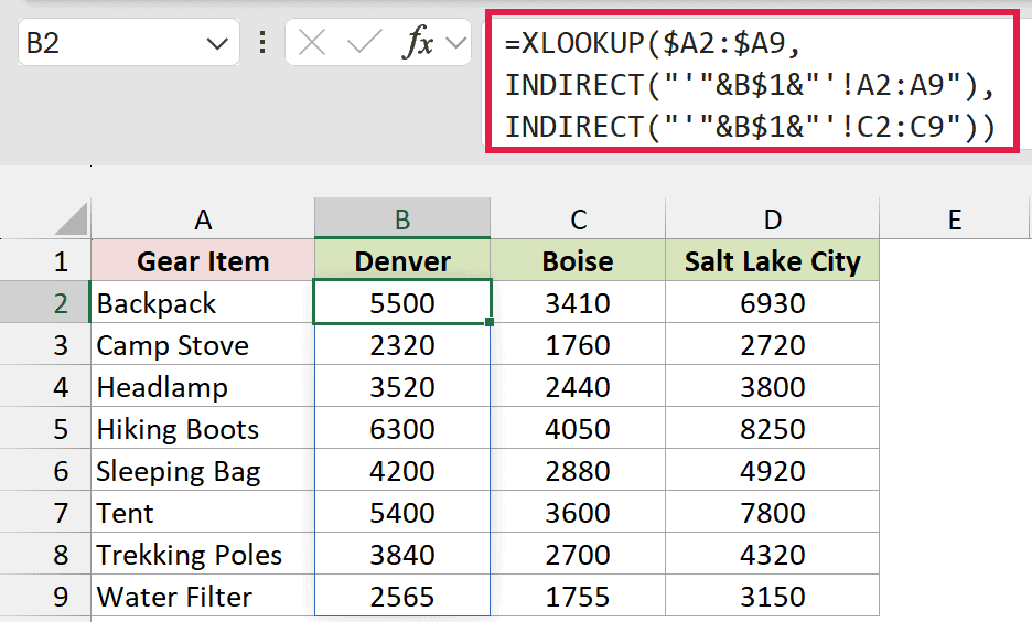
You get each item’s revenue under its store name. For Backpack, you get 5500 for Denver, 3410 for Boise and 6930 for Salt Lake City.
How does this formula work?
XLOOKUP looks up the item names in $A2:$A9. The dollar signs keep column A fixed when the formula is copied to the right.
B$1 reads the sheet name from the header. The dollar sign keeps row 1 fixed while the column letter changes.
The first INDIRECT part points at A2:A9 on that sheet, where XLOOKUP looks for each gear item.
The second INDIRECT part points at C2:C9 on the same sheet. XLOOKUP returns the revenue from that range for each match.
When copied right, B$1 becomes C$1, then D$1. Each column reads its own sheet-name header.
Matching by name means the store sheets can list items in different orders. Backpack’s position on each sheet doesn’t affect the result.
Note: If your Excel version doesn’t support XLOOKUP, you can use the older-Excel formula below. Enter it in B2, then copy across to D2 and down to row 9.
=VLOOKUP($A2,INDIRECT("'"&B$1&"'!A2:C9"),3,FALSE)
You get the same 24 revenue values with this VLOOKUP version.
Method #3: Using the SWITCH Function
If you have a short, fixed list of sheets, I prefer a formula that names each reference directly.
With SWITCH, you can keep those references working when sheets are renamed or rows are inserted.
You can use SWITCH in Excel 2019 and later, or Microsoft 365.
Below I have a dataset of outdoor-gear sales on three sheets named Denver, Boise and Salt Lake City. I keep total revenue in C10 on each sheet.
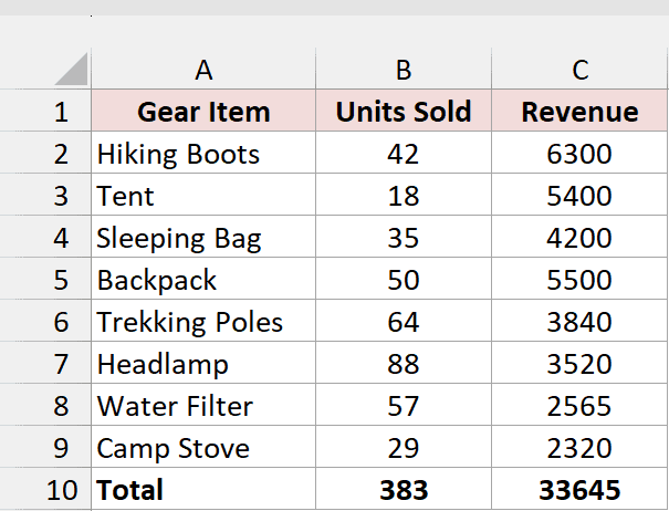
You can see the Denver sheet below, with gear items and their sales in A1:C10.
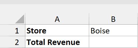
On the SWITCH sheet, I have Store in A1 and Boise in B1. I have Total Revenue in A2, with B2 empty.
You can enter this formula in B2.
=SWITCH(B1,"Denver",Denver!C10,"Boise",Boise!C10,"Salt Lake City",'Salt Lake City'!C10,"Store not found")
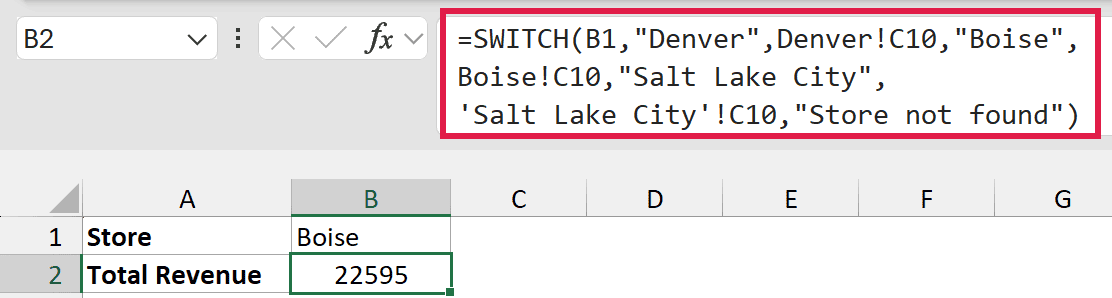
You get 22595, Boise’s total revenue, in B2. You can see the formula in the formula bar.
How does this formula work?
SWITCH compares B1 with each store name in turn and returns the reference paired with the first matching name.
Denver is paired with Denver!C10, Boise with Boise!C10, and Salt Lake City with 'Salt Lake City'!C10.
The final argument, "Store not found", is the result when nothing matches. If you type Seattle in B1, you get that message.
You can also type boise in lowercase and get 22595. The match isn’t case-sensitive.
SWITCH uses normal sheet references that Excel updates for you. Rename Boise to Boise Store, and Excel automatically uses 'Boise Store'!C10. With Boise in B1, you still get 22595.
The matching text “Boise” in the formula stays unchanged. If you’d rather type Boise Store in B1, you’ll need to edit that text in the formula too.
After that rename, both INDIRECT formulas in Methods #1 and #2 return #REF! because your B1 or column header still says Boise, which no longer names a sheet.
Inserting a row above Denver’s Total moves it to C11. Excel updates SWITCH to Denver!C11, so you still get 33645 when you select Denver.
Every sheet must be listed in SWITCH. If you add a new store sheet, you need to edit the formula to include it.
Note: In older Excel, you can select among the same references with CHOOSE and MATCH. Use the formula below. You get #N/A for an unlisted store instead of a message.
=CHOOSE(MATCH(B1,{"Denver","Boise","Salt Lake City"},0),Denver!C10,Boise!C10,'Salt Lake City'!C10)
You get the same store totals for the three listed names.
Additional Notes About Referencing Another Sheet Dynamically in Excel
I keep these details in mind when I use a sheet name from a cell.
- To prevent typos and stray spaces, select B1, then Data tab > Data Tools group > Data Validation. On the Settings tab, set Allow: List, Source
Denver,Boise,Salt Lake City, then click OK. The sample file doesn’t include this drop-down; you add it. - Excel recalculates every INDIRECT formula whenever anything in the workbook changes. That’s called volatility. A handful is fine, but thousands can slow a big workbook. SWITCH isn’t volatile.
- Inserting a row above Denver’s Total moves it to C11. INDIRECT keeps reading C10 and quietly returns 2320, Camp Stove’s revenue, instead of 33645. Its text reference never adjusts, and there’s no error to warn you.
- Keep the same layout on every store sheet so one cell address works for all of them. Total revenue stays in C10 throughout.
Frequently Asked Questions
Here are a few questions people often ask about this.
Why does my INDIRECT formula return #REF!?
You get #REF! when the text doesn’t resolve to a usable reference. These are the usual causes.
- Single quotes are missing around a sheet name containing spaces. Salt Lake City needs them, even though Denver works without them.
- The name has no matching sheet, such as Seattle, or contains leading or trailing spaces. Even
boisereturns #REF!. - The sheet was renamed or deleted, so the name in your input cell no longer matches an existing tab.
- The reference points to another workbook that’s closed.
You can enter boise instead of Boise. Letter case doesn’t matter, but you otherwise need an exact sheet-name match.
Can I make the cell address dynamic too?
You can put the sheet name in B1 and type C10 in B4. I then use this formula to read both inputs.
=INDIRECT("'"&B1&"'!"&B4)
You get the selected store’s total revenue. With Denver in B1, change B4 to B10 and you get 383, its total units sold.
Does INDIRECT work with a different workbook?
You can use INDIRECT to reference another workbook while that file is open. If you close it, you get #REF!.
How do I sum the same cell across all sheets?
You can add C10 across the store sheets with a reference that spans their tabs. I use this 3D reference for the example workbook.
=SUM('Denver:Salt Lake City'!C10)
You get 98130. The reference includes every sheet whose tab sits between Denver and Salt Lake City, including those two endpoints.
Single quotes wrap the whole sheet range, 'Denver:Salt Lake City', because one name contains spaces. Quoting only Salt Lake City returns #NAME?.
This formula adds the same cell across the sheet range, rather than choosing a sheet from an input cell.
Conclusion
I covered INDIRECT for a single cell, INDIRECT with XLOOKUP for a whole range, and SWITCH for a short, fixed list of sheets.
I’d use INDIRECT by default. I hope you found this article helpful.
Other Excel articles you may also like:
- How to Reference a Cell on Another Sheet in Excel
- How to VLOOKUP Between Two Sheets in Excel (4 Easy Ways)
- Get a List of All Sheet Names in Excel (3 Easy Ways)
- How to Get Excel Sheet Names? (3 Easy Ways)
- ISREF Function in Excel (4 Easy Examples)
- XLOOKUP vs VLOOKUP in Excel (7 Examples)
- How to Link Cells in Excel (Same Worksheet, Between Worksheets/Workbooks)
- How to Create a Dynamic Named Range in Excel (4 Easy Ways)
