How to Build an Amortization Schedule with Irregular Payments in Excel

An amortization schedule in Excel shows how each loan payment splits between interest and principal, and how fast the balance drops. That’s simple when every payment is the same, but real payments are rarely that tidy.

You might throw an extra $1,000 at the loan after a bonus, skip a month when money is tight, or pay on whatever date you have the cash. Each of those changes the balance, and every interest charge after it.

The catch is that Excel’s built-in loan functions, like IPMT and PPMT, assume you pay the same amount every period. So a schedule with irregular payments has to work row by row, charging interest on whatever balance is actually left.

In this article, I’ll show you how to add an extra payment column (and see how much interest it saves), track variable and skipped payments, calculate interest for payments on irregular dates, and build the whole schedule with one SCAN formula.

Method #1: Using an Extra Payment Column

This is the method I’d use for most loans. You keep the regular monthly payment, and add a column where you type any extra amount you pay on top of it.

Below I have a $9,000 personal loan at 12% annual interest over 18 months. The loan details are in A1:B4, and the schedule below them lists the months, with the extra payments I plan to make in column D.

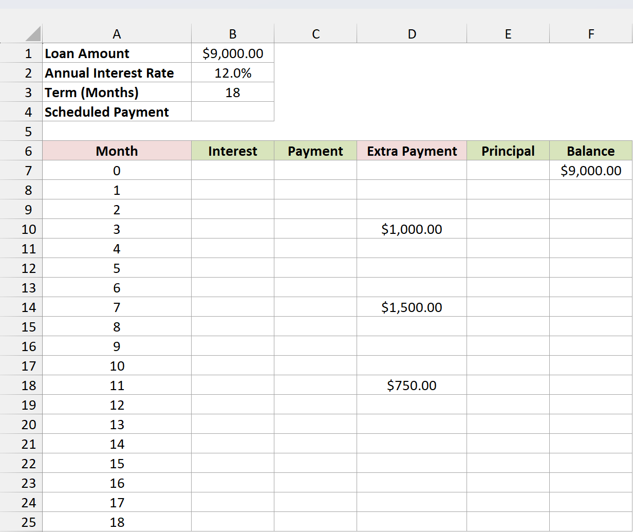
Row 7 is month 0, the day the loan starts. Its Balance cell (F7) holds =$B$1, so the schedule begins at the full loan amount.

First, let’s work out the regular monthly payment. Here is the formula I entered in B4:

=PMT(B2/12,B3,-B1)

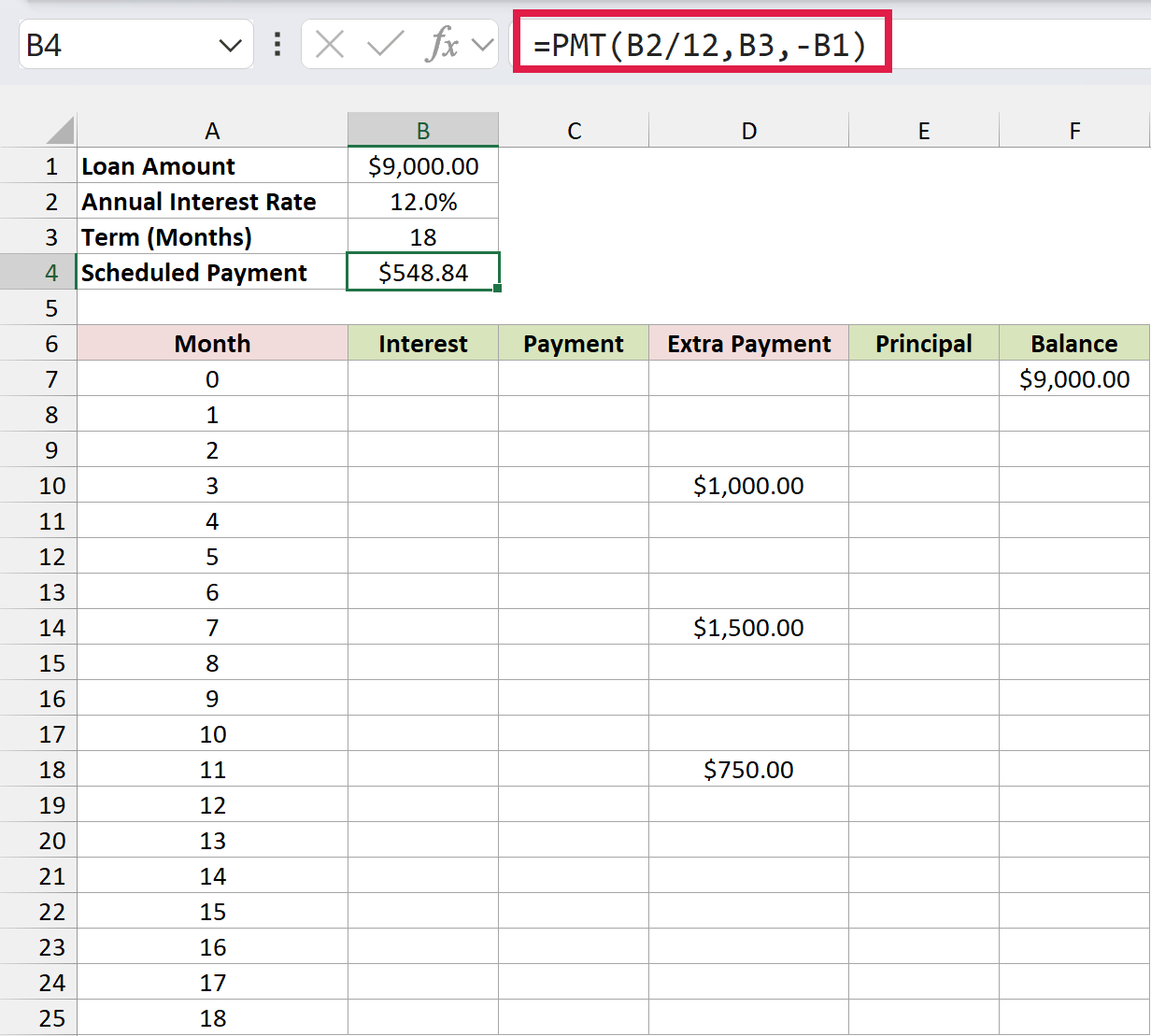
The PMT function returns $548.84.

B2/12 turns the 12% annual rate into a 1% monthly rate, B3 is the number of payments. The minus sign in front of B1 makes the result positive, since PMT otherwise returns a payment as a negative number (money going out).

Now let’s fill in month 1. Here is the formula for the interest in B8:

=F7*$B$2/12

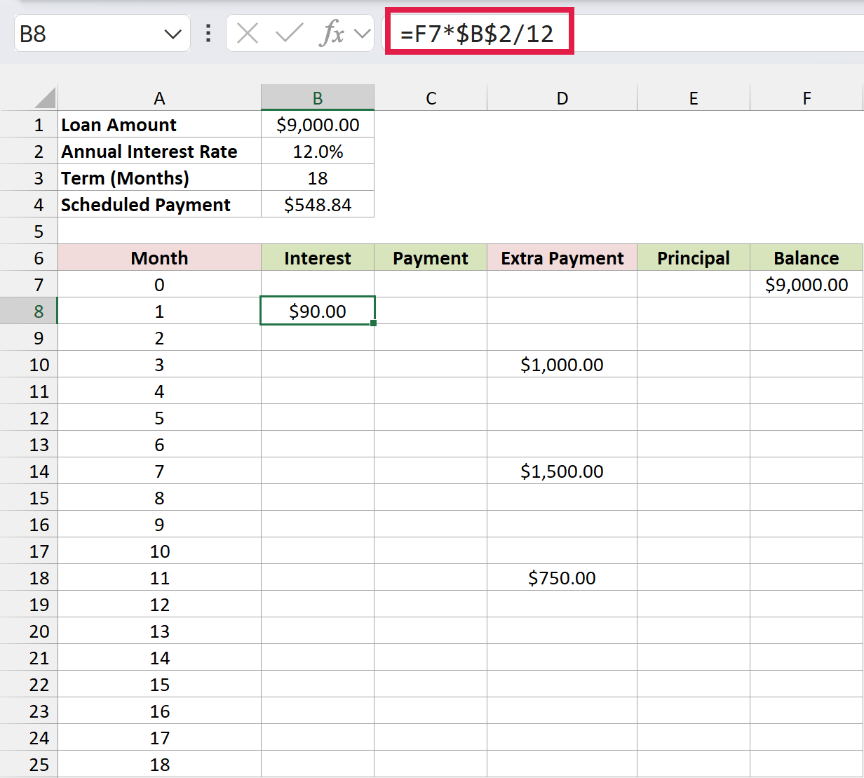
This takes last month’s balance in F7 and multiplies it by the monthly rate. The first month’s interest is $90.00, which is 1% of $9,000.

Next, the regular payment. Here is the formula in C8:

=MIN($B$4,F7+B8)

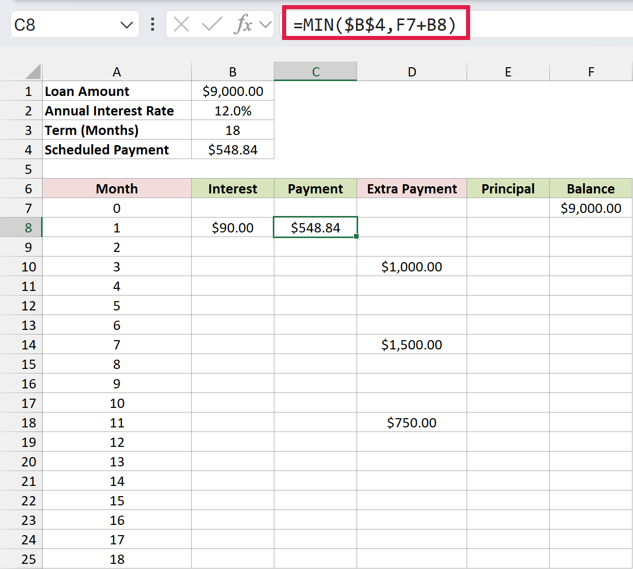
Most months, this returns the scheduled $548.84. But the MIN function also compares it with what you actually owe (last balance plus this month’s interest) and returns the smaller one. That way, the final payment is only what’s left, not a full $548.84.

Now the principal. Here is the formula in E8:

=MIN(C8-B8+D8,F7)

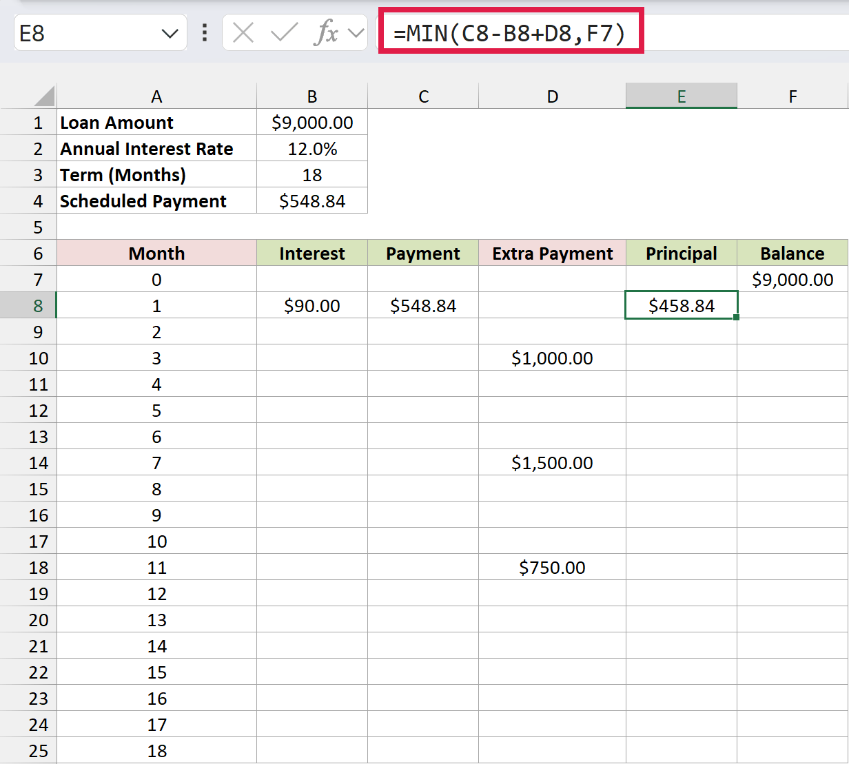
How does this formula work?

C8-B8 is the part of the regular payment left after interest. Adding D8 puts any extra payment straight toward principal. In month 1 there’s no extra, so the principal is $458.84.

The MIN part caps the principal at last month’s balance in F7. So if an extra payment is bigger than what you still owe, the balance stops at zero instead of going negative.

The last formula for month 1 is the new balance. Here is the formula in F8:

=F7-E8

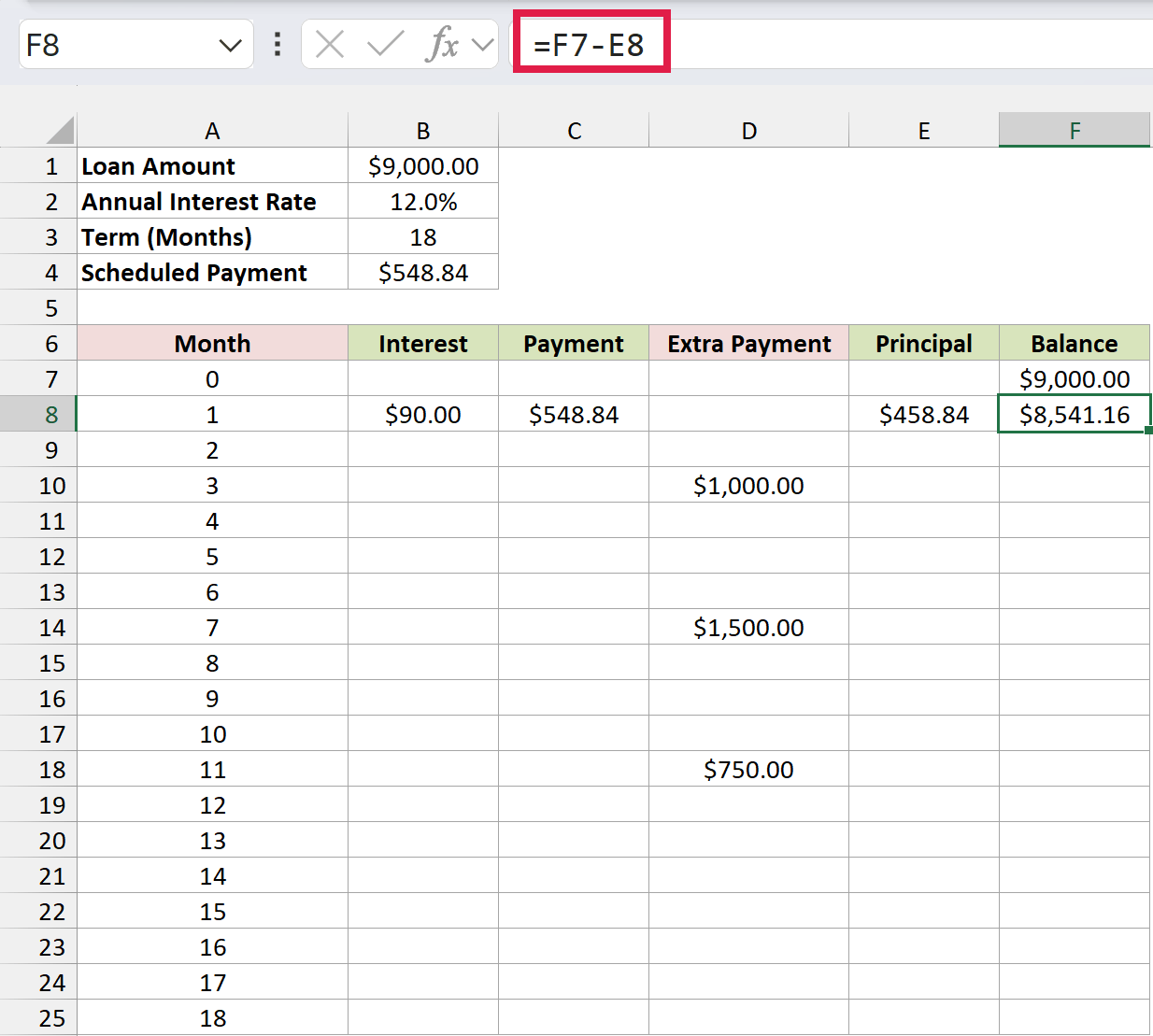
The balance after month 1 is $8,541.16.

Every formula in row 8 points at the row above it, so you can’t replace them with one spilling formula. Instead, copy them down the schedule. Here are the steps:

1. Copy B8:C8, select B9:C25, and paste.
2. Copy E8:F8, select E9:F25, and paste.

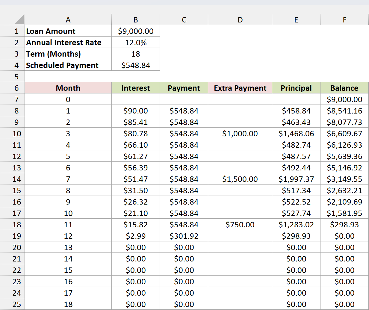
I copied the two pairs separately so the extra payments in column D don’t get overwritten.

Look at months 3, 7, and 11. The principal jumps on each of those rows because the extra payment goes straight to the balance. The loan is paid off in month 12, where the payment drops to $301.92, and every month after that shows $0.00.

Note: Column D shows what you typed, not what was applied. If you enter an extra payment larger than the remaining balance, the Principal formula only applies what’s needed to reach zero, so check the last month before you send the money.

Now let’s see what those extra payments actually saved. I added three labels in H1:H3. Here is the formula for the total interest paid in I1:

=SUM(B8:B25)

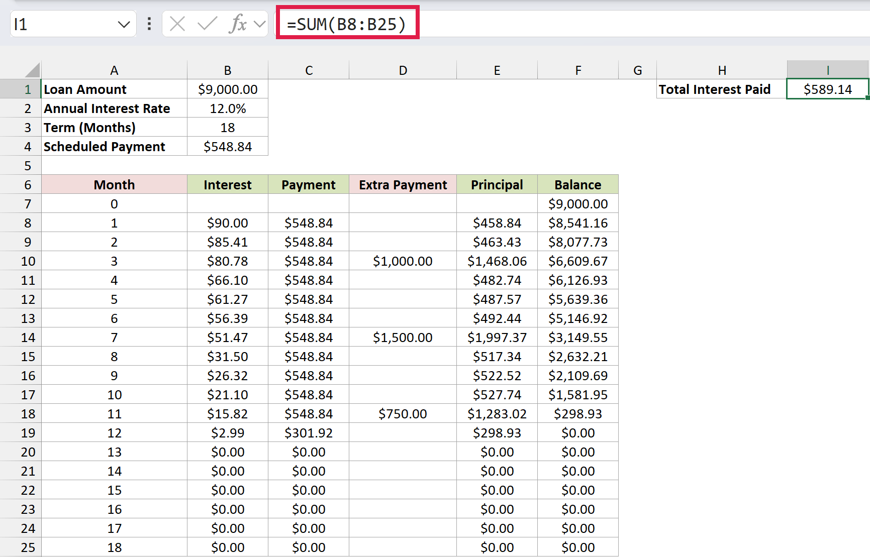
With the extra payments, the loan costs $589.14 in interest.

To compare that with the regular schedule, here is the formula for the interest saved in I2:

=B4*B3-B1-I1

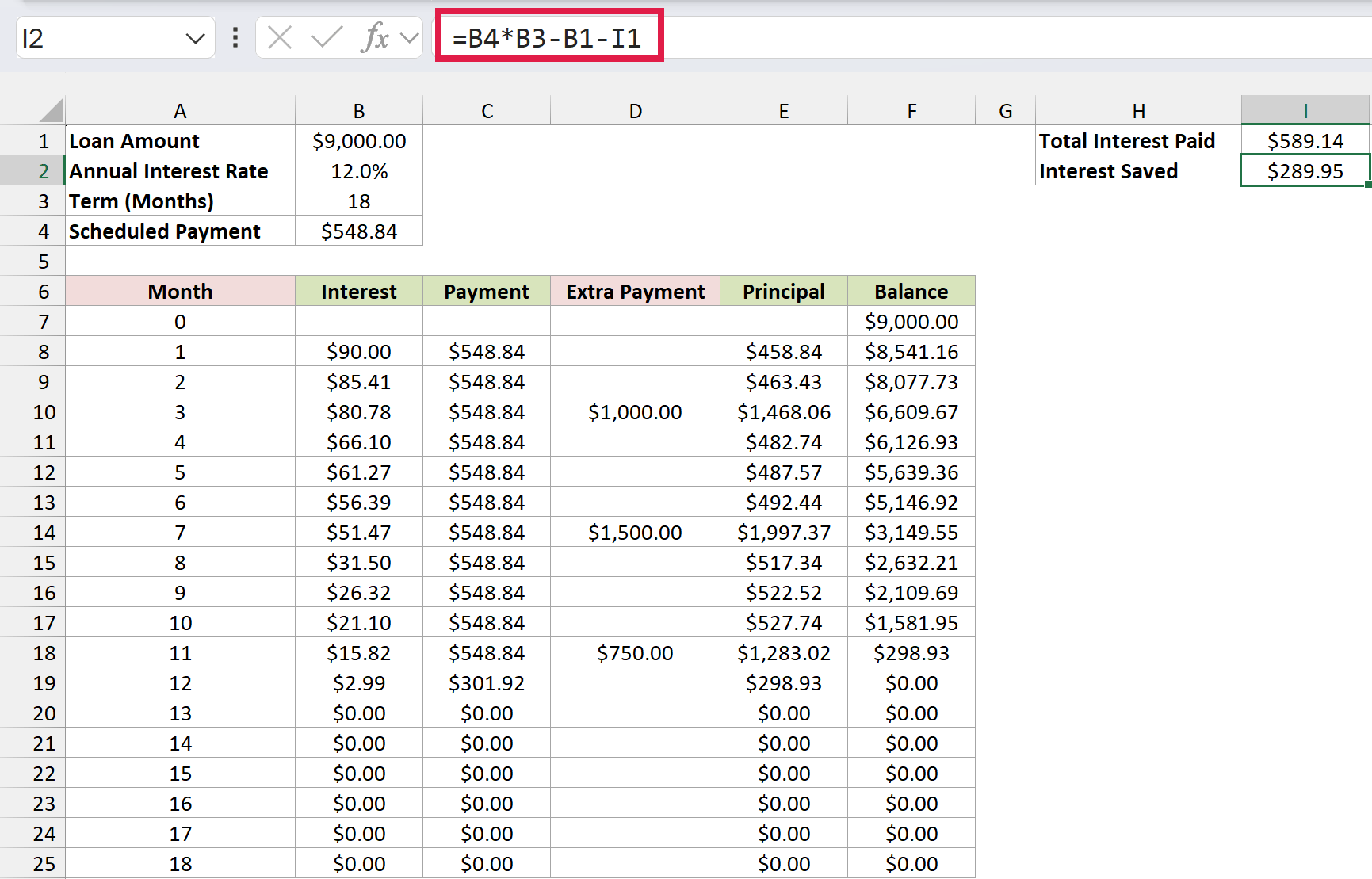
B4*B3 is what 18 regular payments add up to. Subtracting the $9,000 loan leaves the interest you’d pay with no extras, which is $879.09. Take away the interest you actually pay in I1, and the extra payments save you $289.95.

Finally, here is the formula for the months saved in I3:

=B3-COUNTIF(E8:E25,">0")

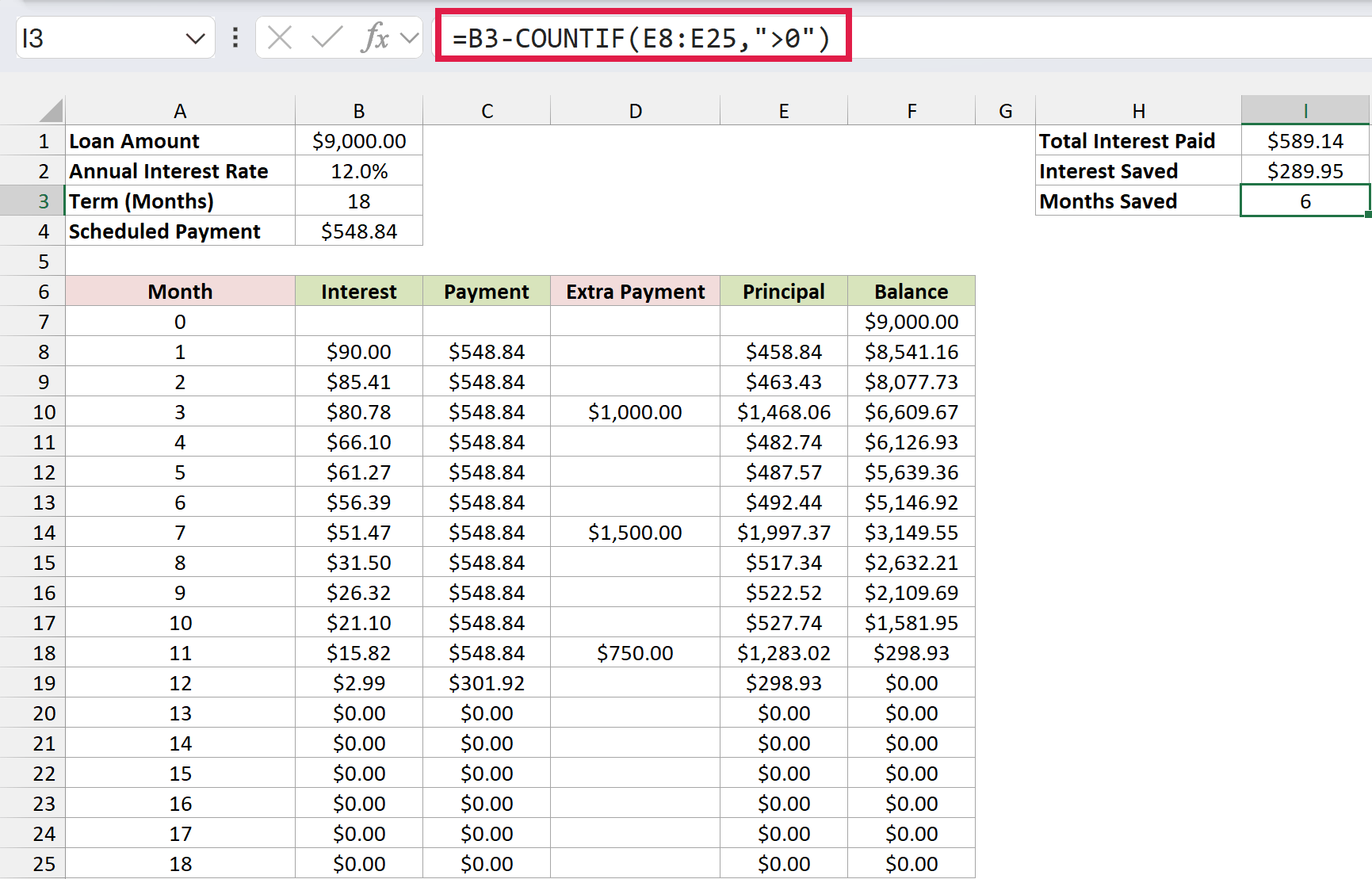
The COUNTIF function counts the months where some principal was paid, which is 12. The loan term is 18 months, so you’re done 6 months early.

The schedule updates the moment you change anything. Type a new amount in column D, and the balance, payoff month, and savings all recalculate.

Method #2: Using an Actual Payment Column

If your loan doesn’t have a fixed payment, this one is for you. It works well for a flexible loan, like one from a family member, where you pay what you can each month and sometimes skip a month entirely.

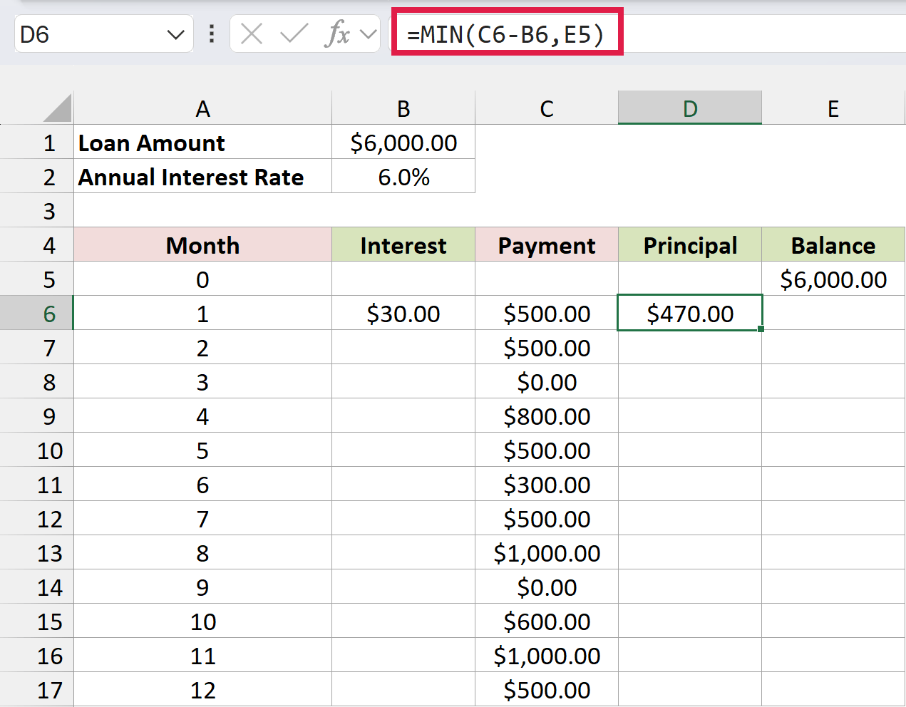
Below I have a $6,000 loan at 6% annual interest. Instead of a calculated payment, column C has what was actually paid each month, including two skipped months with $0.

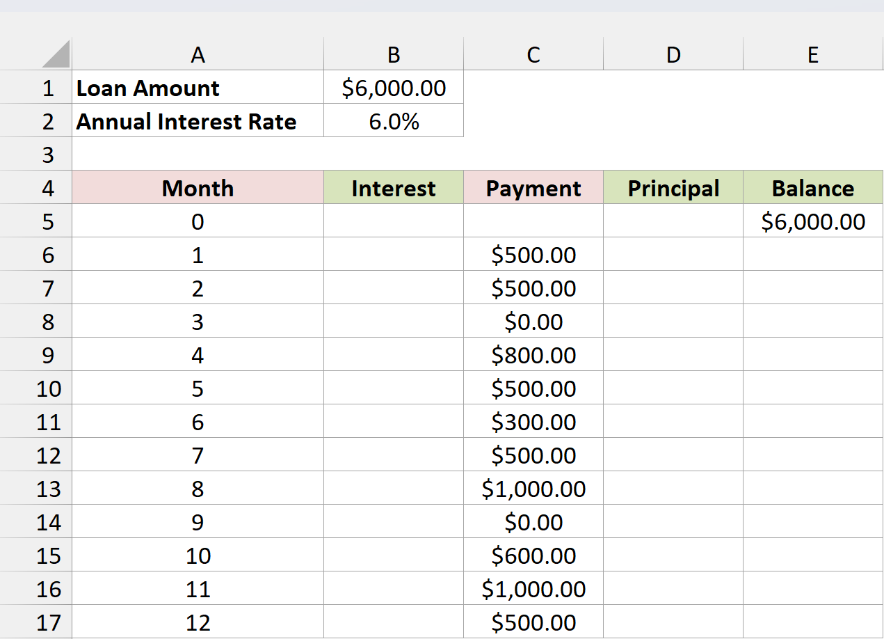
Month 0 is in row 5, and its Balance cell (E5) holds =$B$1, the starting loan amount.

Let’s start with the interest for month 1. Here is the formula in B6:

=E5*$B$2/12

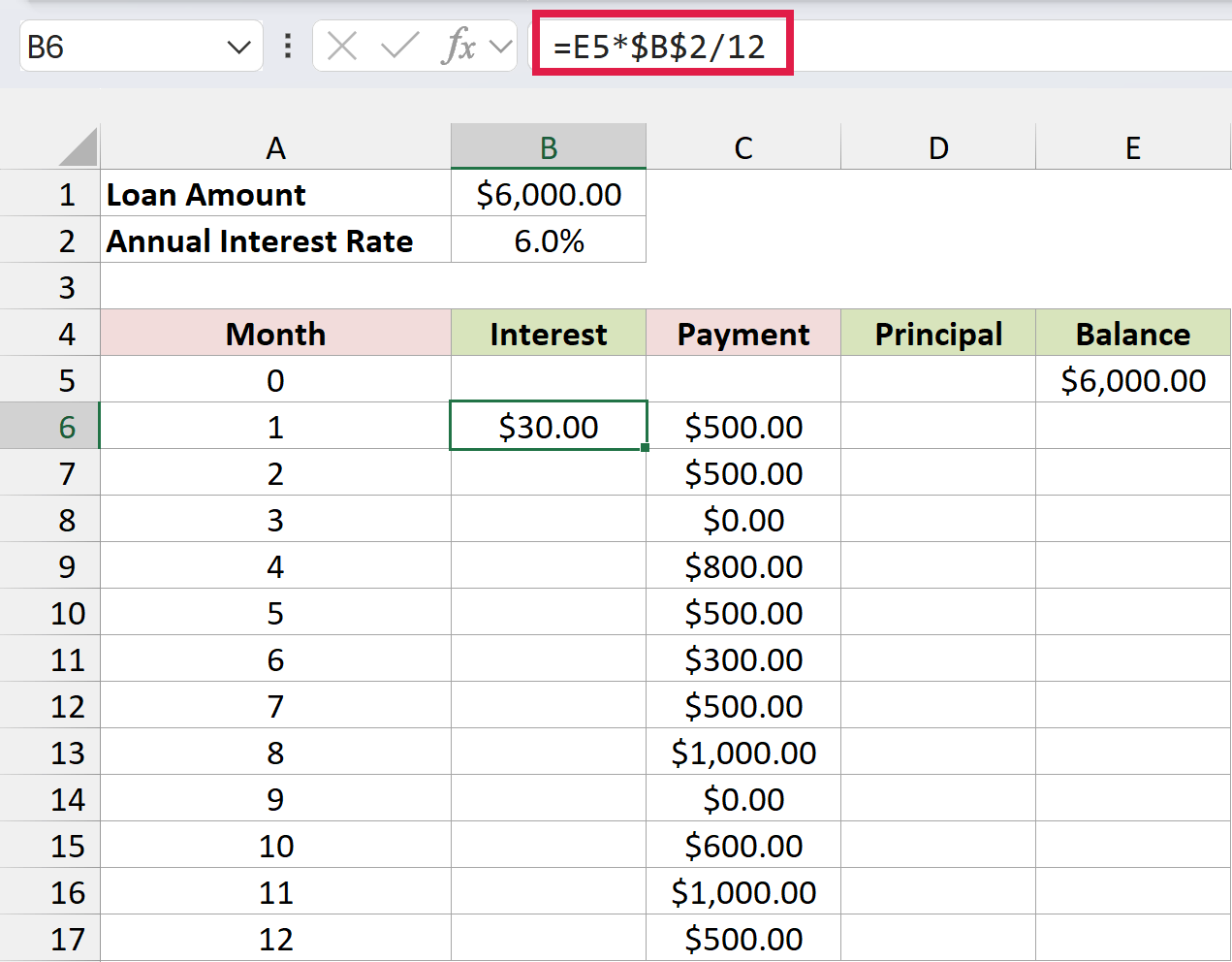
At 6% a year, the monthly rate is 0.5%, so the first month’s interest on $6,000 is $30.00.

Next, the principal. Here is the formula in D6:

=MIN(C6-B6,E5)

How does this formula work?

C6-B6 is whatever is left of the payment after interest. In month 1, that’s $500 minus $30, so $470 goes toward the loan.

When a payment is skipped, C is $0, so the principal comes out negative. That’s correct, because the unpaid interest gets added to what you owe.

The MIN part caps the principal at last month’s balance, so an overpayment in the final month can’t push the balance below zero.

Now the new balance. Here is the formula in E6:

=E5-D6

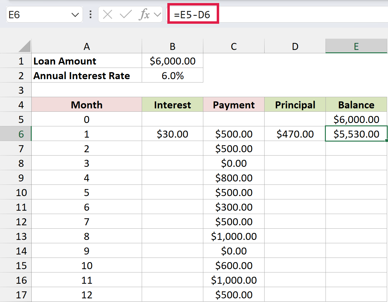
The balance after month 1 is $5,530.00.

These formulas also depend on the row above, so copy them down the schedule. Here are the steps:

1. Copy B6, select B7:B17, and paste.
2. Copy D6:E6, select D7:E17, and paste.

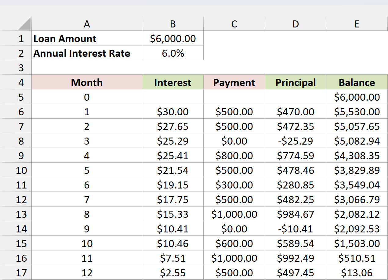
Look at month 3. Nothing was paid, so the principal is -$25.29 and the balance grows from $5,057.65 to $5,082.94. The same thing happens in month 9. After 12 months, $13.06 is still owed.

Note: This schedule only adds the unpaid interest for a skipped month. Many lenders also charge a late fee, so add that to the balance yourself if your loan has one.

Method #3: Using Daily Interest for Irregular Dates

The first two methods assume one payment a month. If you pay on irregular dates instead, the interest depends on how many days passed since the last payment.

Below I have a $7,500 loan at 7.3% annual interest. Row 5 has the date the loan started (2/1/2026), and each row after it has a payment date and the amount paid.

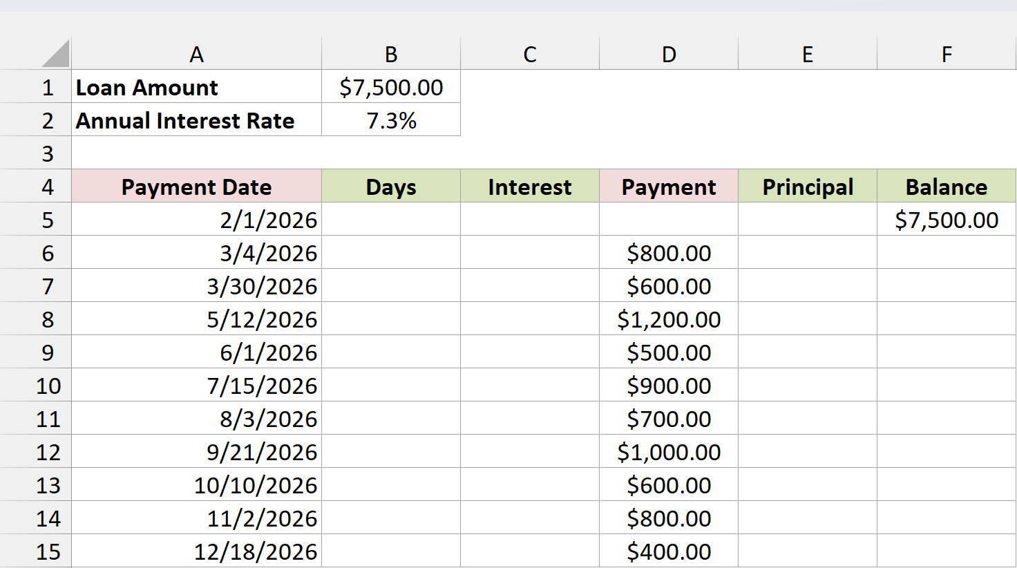
The Balance cell in row 5 (F5) holds =$B$1, so the schedule starts at the full $7,500. Make sure the dates are in order, oldest first, because every formula looks at the row above.

First, let’s count the days since the last payment. Here is the formula in B6:

=A6-A5

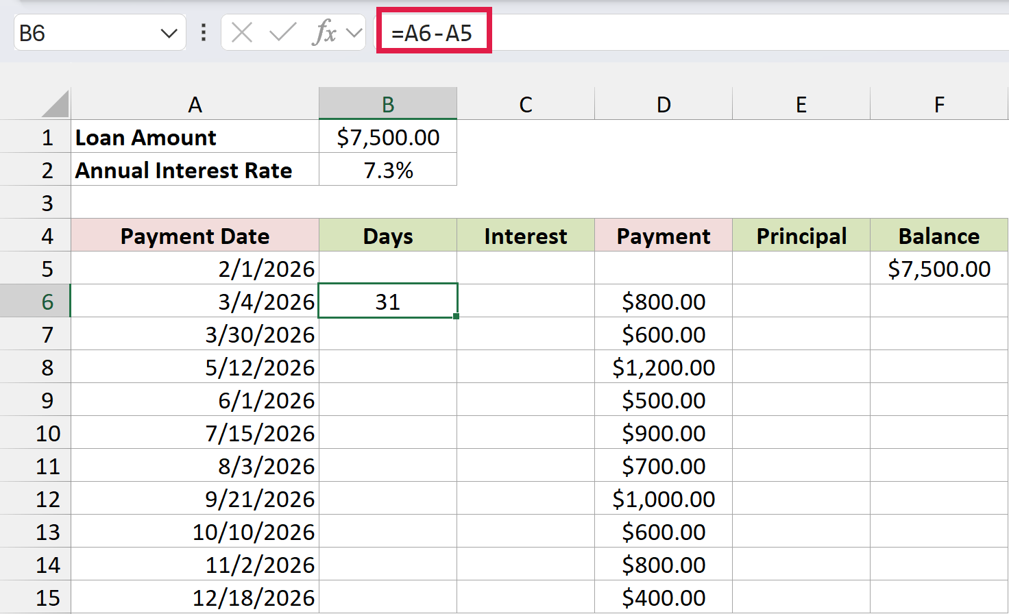
Excel stores dates as numbers, so subtracting one date from another returns the number of days between them. It’s 31 days from 2/1/2026 to 3/4/2026.

Next, the interest for those days. Here is the formula in C6:

=F5*$B$2*B6/365

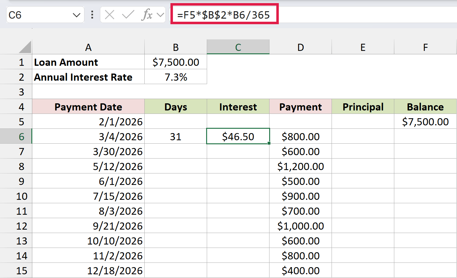
How does this formula work?

$B$2/365 is the daily rate. At 7.3% a year, that’s 0.02% a day, which keeps the math easy to check.

The formula multiplies last balance by the daily rate, then by the number of days. So 31 days on $7,500 comes to $46.50. A payment made after 43 days carries more interest than one made after 19 days.

Now the principal. Here is the formula in E6:

=MIN(D6-C6,F5)

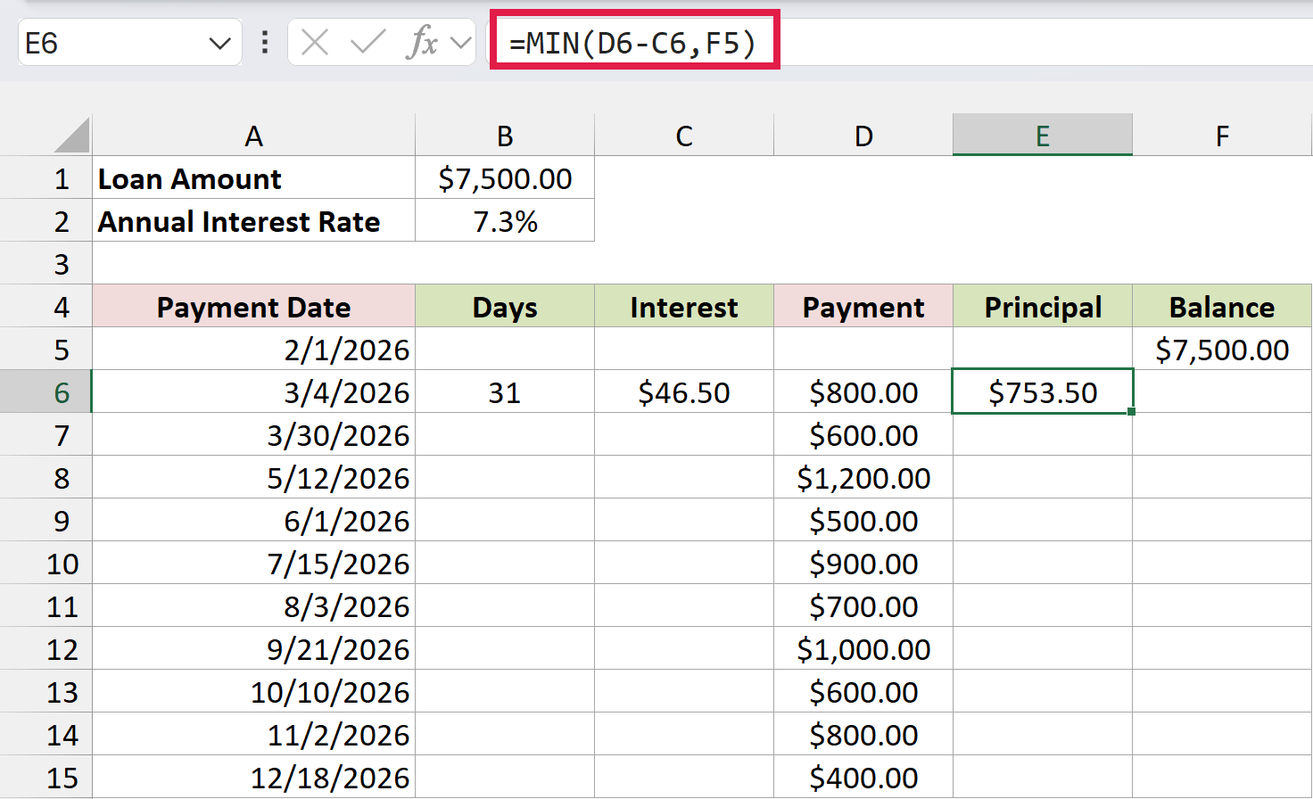
This works just like Method #2. The payment minus the interest goes to principal, capped at the last balance. For the first payment, that’s $753.50.

And the new balance. Here is the formula in F6:

=F5-E6

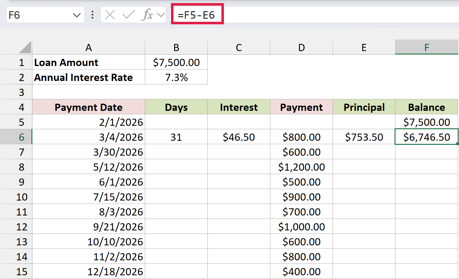
Now copy everything down the schedule. Here are the steps:

1. Copy B6:C6, select B7:C15, and paste.
2. Copy E6:F6, select E7:F15, and paste.

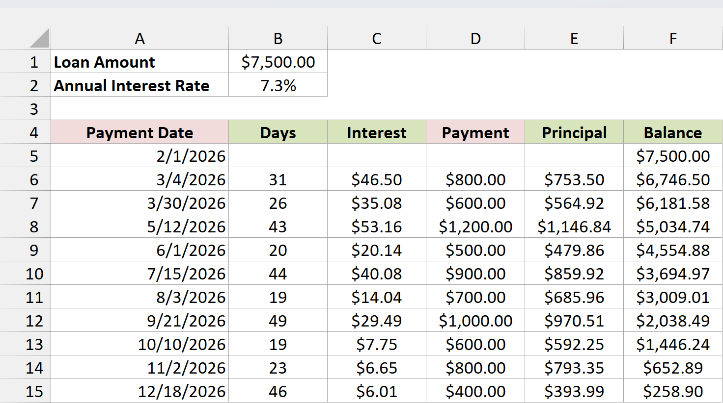
After 10 payments, the balance is $258.90. Notice how the interest changes with the gap between payments, from $7.75 after 19 days to $53.16 after 43 days.

Note: If the Days column shows a date like 1/31/1900 instead of a number, Excel copied the date format into it. Select the column and change the format to General or Number.

This daily method matches simple-interest loans, like many personal and auto loans. A standard mortgage usually charges a full month of interest no matter which day you pay, so Method #1 fits it better.

Method #4: Using the SCAN Function

If you have Excel for Microsoft 365 or Excel 2024, you can skip the copy-down step completely. One formula takes the list of payments and spills the interest, principal, and balance for every month.

Below I have the same $6,000 loan at 6% from Method #2, with the payments for 12 months in column B (including the two skipped months).

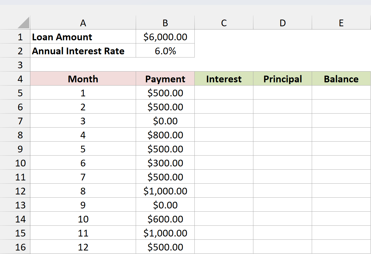
Here is the formula I entered in C5:

=LET(loan,$B$1,mRate,$B$2/12,pays,B5:B16,bal,SCAN(loan,pays,LAMBDA(prev,pay,MAX(0,prev*(1+mRate)-pay))),opening,VSTACK(loan,DROP(bal,-1)),interest,opening*mRate,HSTACK(interest,opening-bal,bal))

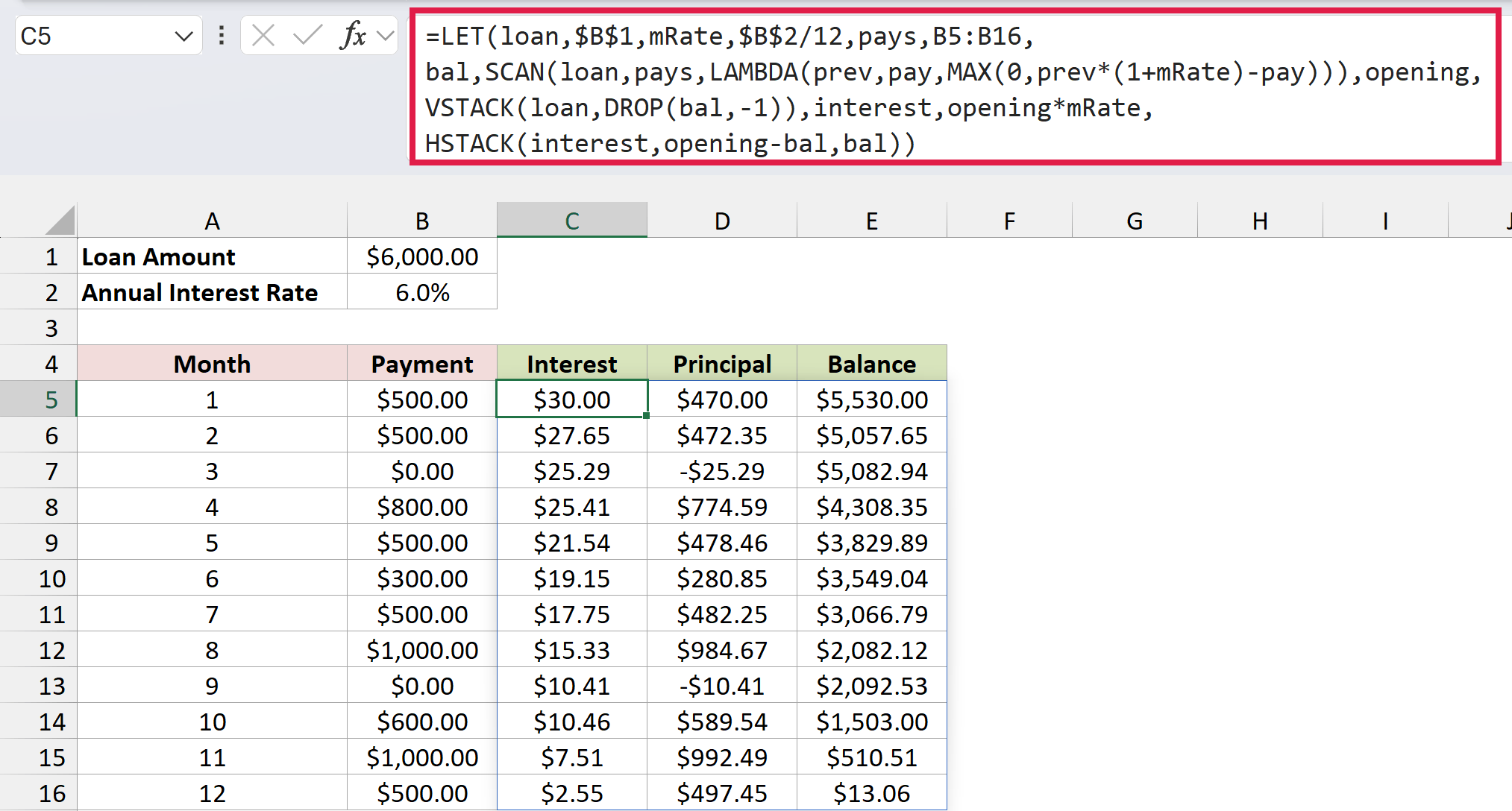
The formula spills across C5:E16, and every number matches the schedule from Method #2 to the cent.

How does this formula work?

The LET function gives names to the pieces so the formula is easier to read. loan is the $6,000, mRate is the monthly rate, and pays is the list of payments.

The SCAN function does the real work. It starts with the loan amount and goes down the payments one at a time.

For each payment, it adds a month of interest to the previous balance, subtracts the payment, and keeps the result. MAX(0, …) stops the balance from going below zero. That gives a list of the balances after each month, called bal.

opening is the balance at the start of each month. VSTACK puts the loan amount on top of the bal list, and DROP removes the last balance so the list stays 12 rows long. interest is each opening balance times the monthly rate.

Finally, HSTACK puts three columns side by side: the interest, the principal (opening balance minus closing balance), and the balance.

Note: SCAN, LAMBDA, VSTACK, HSTACK, and DROP need Excel for Microsoft 365 or Excel 2024. The formula also needs three empty columns to spill into, or it returns a #SPILL! error.

To change a payment, type a new amount in column B, and the whole schedule recalculates.

Additional Notes About Amortization Schedules with Irregular Payments in Excel

• Your lender’s numbers may be a few cents off. Lenders round interest to the cent every period, while these formulas keep full precision. Wrap the interest formula in ROUND, like =ROUND(F7*$B$2/12,2), to match a statement more closely.
• Ask how your lender applies extra payments. Some put extra money toward principal right away. Others treat it as an early payment of next month’s installment, which saves much less interest.
• Some loans use a 360-day year. If your loan agreement says so, change the 365 in Method #3 to 360.
• Keep enough rows for the full term. In Method #1, the schedule runs all 18 months even though the loan ends sooner. If you lower the extra payments, the later rows are already there to show the longer payoff.

Frequently Asked Questions

Here are some common questions about irregular payments in an Excel amortization schedule.

Can I use IPMT and PPMT for a schedule with extra payments?

No. The IPMT and PPMT functions calculate interest and principal from the original loan terms, assuming the same payment every period. After the first extra payment, their numbers no longer match the real balance.

How do I hide the rows after the loan is paid off?

Select the header row of the schedule and press Ctrl + Shift + L to add filter arrows. Then filter the Payment column to uncheck $0.00. The rows are hidden, not deleted, so they come back if the payoff date moves.

How do I add the same extra payment every month?

Type the amount in the first Extra Payment cell (D8 in Method #1), then copy it down the column. You can still overwrite any single month with a different amount.

Does paying extra lower my monthly payment?

Not in this schedule. The regular payment stays at $548.84, and the loan ends sooner. Some lenders will recalculate a lower payment after a large lump sum (called recasting), but that’s something you arrange with them.

What if the interest rate changes partway through the loan?

Add an Annual Rate column to the schedule, type each month’s rate in it, and point the Interest formula at that column instead of $B$2. For example, with the rate in column G, the interest in B8 becomes =F7*G8/12.

Conclusion

An amortization schedule with irregular payments needs each row to start from the real balance left after the last payment. For most loans, I’d go with the extra payment column from Method #1, since it also shows how much interest and time you save.

If your payments change every month, or land on irregular dates, Methods #2 and #3 handle that. And if you have Excel for Microsoft 365 or Excel 2024, the SCAN formula builds the same schedule in one go. I hope you found this article helpful.

Other Excel articles you may also like:

• How to Build a Car Loan Amortization Schedule in Excel
• How to Build a Mortgage Calculator in Excel
• Loan Amortization Schedule Calculator
• Calculate Credit Card Interest in Excel (Free File Download)
• How to Calculate Simple Interest in Excel (5 Easy Ways)
• CUMIPMT Function in Excel (6 Easy Examples)
• NPER Function in Excel (5 Easy Examples)
• How to Loop in Excel Formulas Without VBA (6 Easy Ways)