
Simple interest is the easy kind of interest to work out in Excel.
You multiply the principal by the annual rate and the time, and interest is only ever charged on the original amount.
The math is always the same, but the time can come to you as a number of years, a number of months, or a start date and an end date.
Dates are where people get different answers for the same loan. It depends on whether a year counts as 360 days, 365 days, or twelve 30-day months.
In this article, I’ll show you how to calculate simple interest from years, months, and dates. I’ll also cover picking the day-count basis with YEARFRAC and working backward to the rate, time, or principal.
Method #1: Using the P*R*T Formula
The simple interest formula is Principal × Rate × Time. When the time is already in years, you can type it into Excel almost exactly like that.
Below I have a dataset on the Known Years sheet. Column A has the purpose of each loan, and columns B to D have the principal, annual rate, and term in years.
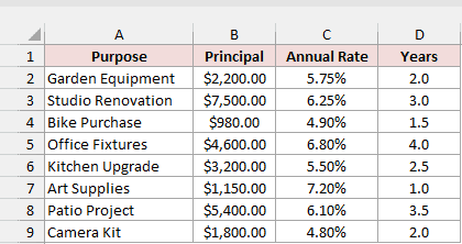
I want to calculate the interest for each loan in column E.
Here is the formula to enter in E2:
=B2:B9*C2:C9*D2:D9
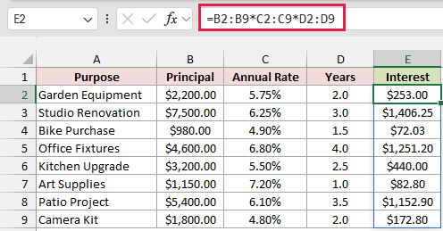
The formula spills down the column automatically. For Garden Equipment, $2,200 at 5.75% for 2 years returns $253.00 in interest.
How does this formula work?
Excel multiplies the three columns row by row, so each loan gets its own principal × rate × years.
The years don’t have to be whole numbers. Bike Purchase runs 1.5 years and returns $72.03.
Range formulas like this spill in Excel 2021, Excel 2024, and Microsoft 365. In Excel 2019 or earlier, enter =B2*C2*D2 in E2 and copy it down to E9.
Now let’s get the total amount due, which is the principal plus the interest.
Here is the formula to enter in F2:
=B2:B9*(1+C2:C9*D2:D9)
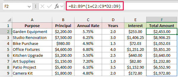
For Garden Equipment, the total amount is $2,453.00, which is the $2,200 principal plus the $253.00 interest.
This is the P × (1 + R × T) version of the formula, so it doesn’t need the interest column at all.
If you already have column E, =B2:B9+E2# returns the same totals.
Note: Enter the rate as a percentage (5.75%) or as a decimal (0.0575). If you type 5.75 as a plain number, Excel treats it as 575%, and the Garden Equipment interest becomes 25,300 instead of 253.
Method #2: Using a Month Count (Months ÷ 12)
A lot of short loans and deposits are quoted in months, not years. The rate is still annual, so you just turn the months into years before multiplying.
Below I have a dataset on the Months sheet. Column A has each borrower, and columns B to D have the principal, annual rate, and term in months.
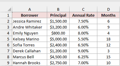
I want the interest for each borrower in column E.
Here is the formula to enter in E2:
=B2:B9*C2:C9*(D2:D9/12)
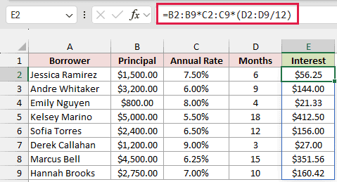
The results spill down the column. Jessica Ramirez borrows $1,500 at 7.5% for 6 months, so her interest is $56.25.
How does this formula work?
D2:D9/12 turns each month count into a fraction of a year. Six months becomes 0.5, and 18 months becomes 1.5.
Then it’s the same principal × rate × time as Method #1. If you’d rather think in a monthly rate, =B2:B9*(C2:C9/12)*D2:D9 gives exactly the same results.
Method #3: Using the Date Difference (Days ÷ 365)
When a loan runs between two dates, the time is the number of days divided by the days in a year.
Excel stores dates as numbers, so subtracting one date from another gives you the days.
Below I have a dataset on the Date Interval sheet. Column A has the loan ID, columns B and C have the principal and annual rate, and columns D and E have the start and end dates.
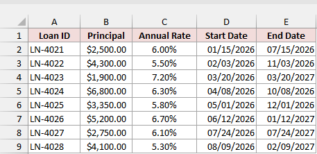
I want the interest for each loan in column F, counting the actual days and a 365-day year.
Here is the formula to enter in F2:
=B2:B9*C2:C9*(E2:E9-D2:D9)/365
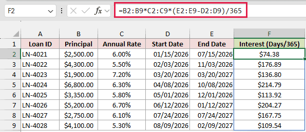
The formula spills down the column. For loan LN-4021, which runs from January 15 to July 15, 2026, it returns $74.38 in interest on $2,500 at 6%.
How does this formula work?
E2:E9-D2:D9 returns the days in each loan. LN-4021 has 181 days, and LN-4023 runs exactly one year, so it has 365.
Dividing by 365 turns the days into a fraction of a year, and the rest is principal × rate × time. This is also the formula for daily simple interest.
Method #4: Using the YEARFRAC Function
Not every agreement uses actual days over 365. Some count every month as 30 days, and some divide by 360.
The YEARFRAC function returns the fraction of a year between two dates, using the day-count basis you choose.
Below I have the same loan dataset on the Date Interval sheet, with the principal, annual rate, start date, and end date in columns B to E.
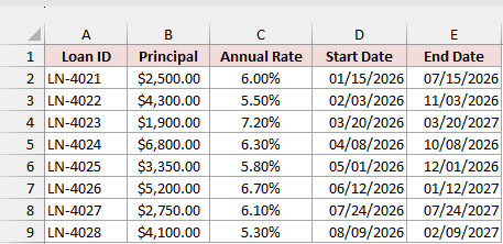
I want to calculate the interest with YEARFRAC in column G.
Here is the formula to enter in G2 and copy down to G9:
=B2*C2*YEARFRAC(D2,E2,3)
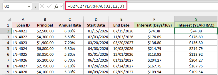
Every row matches column F. LN-4021 returns $74.38 again, because basis 3 means Actual/365.
This one is a per-row formula because YEARFRAC doesn’t accept ranges. =YEARFRAC(D2:D9,E2:E9,3) returns a #VALUE! error instead of spilling.
How does this formula work?
YEARFRAC(D2,E2,3) returns 181/365 of a year for LN-4021. Multiplying that by the principal and the rate gives the interest.
The last argument is the basis. Always type it. If you leave it out, YEARFRAC uses US (NASD) 30/360, and LN-4021 returns $75.00 instead of $74.38.
To see the difference the basis makes, below I have a $25,000 loan at 8% from March 1 to September 1, 2026 on the Day-Count Basis sheet. Bases 0 to 3 are listed in A7:A10.
Here is the formula to enter in C7 and copy down to C10:
=$B$1*$B$2*YEARFRAC($B$3,$B$4,A7)
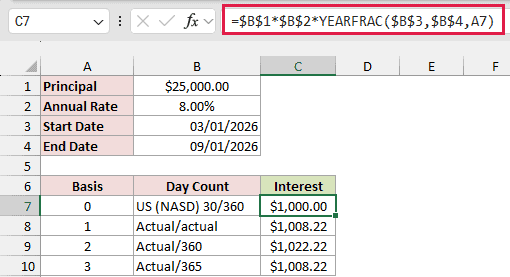
The same loan returns $1,000.00 on 30/360, $1,008.22 on Actual/365, and $1,022.22 on Actual/360. That’s a $22.22 spread from the basis alone.
Basis 0 counts every month as 30 days, the same way the DAYS360 function does, so March to September is exactly 180 days.
Actual/actual matches Actual/365 here because 2026 isn’t a leap year.
Method #5: Using the ACCRINTM Function
Excel doesn’t have a function called SIMPLEINTEREST, but the ACCRINTM function comes close.
It returns the interest on a security that pays all its interest at maturity, which is simple interest on the principal.
Below I have the same loan dataset on the Date Interval sheet, with the principal, annual rate, start date, and end date in columns B to E.
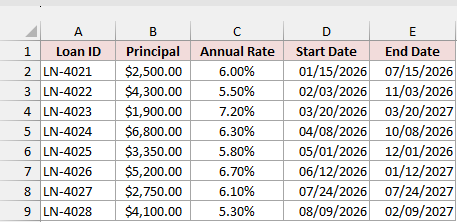
I want the interest from ACCRINTM in column H.
Here is the formula to enter in H2 and copy down to H9:
=ACCRINTM(D2,E2,C2,B2,3)
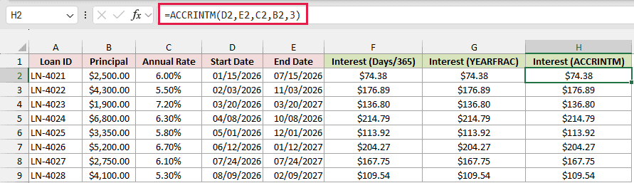
Every row matches columns F and G. LN-4021 returns $74.38 once more.
Like YEARFRAC, ACCRINTM doesn’t accept ranges, so it’s a per-row formula. A range version returns #VALUE!.
How does this formula work?
The arguments go start date, end date, rate, principal, then basis.
Notice the dates come first and the principal comes last, which is the opposite of the P × R × T order.
ACCRINTM multiplies the principal by the rate and by the days over the year basis. Basis 3 is Actual/365, so it lands on the same number as Method #3.
Note: The basis defaults to 30/360 in ACCRINTM too, so leaving out the 3 returns $75.00 for LN-4021. ACCRINTM also returns #NUM! if the start date isn’t earlier than the end date.
Finding the Rate, Time, or Principal in Simple Interest
Sometimes you know the interest and need one of the other numbers. Since interest is principal × rate × time, you divide the interest by the two numbers you know.
Below I have a card on the Find Rate, Time, Principal sheet with the principal in B1, the years in B2, and the interest in B3.
I want the annual rate in B4.
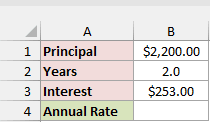
Here is the formula to enter in B4:
=B3/(B1*B2)
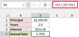
$253 of interest on $2,200 over 2 years means an annual rate of 5.75%. Format B4 as a percentage so it doesn’t show as 0.0575.
The second card has the principal in B6, the annual rate in B7, and the interest in B8. To find the years, enter this formula in B9:
=B8/(B6*B7)
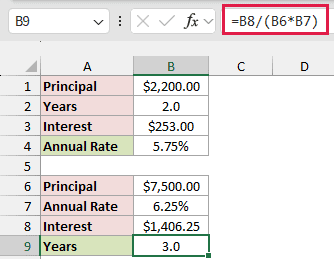
$1,406.25 of interest on $7,500 at 6.25% means the loan ran for 3.0 years.
The third card has the annual rate in B11, the years in B12, and the interest in B13. To find the principal, enter this formula in B14:
=B13/(B11*B12)
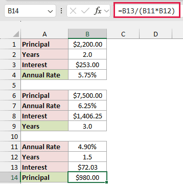
$72.03 of interest at 4.9% over 1.5 years means the principal was $980.00.
Additional Notes About Calculating Simple Interest in Excel
- An annual rate needs the time in years. If you forget to divide months by 12, Jessica Ramirez’s interest jumps from $56.25 to $675.00.
- Currency formatting changes only what you see, not the stored value. LN-4021 displays as $74.38 but is stored as 74.3835616… If you need the stored value in cents, wrap the formula in ROUND:
=ROUND(B2:B9*C2:C9*(E2:E9-D2:D9)/365,2). - Methods #1 to #3 use range formulas that spill in Excel 2021, Excel 2024, and Microsoft 365. In Excel 2019 or earlier, enter the one-row version (like
=B2*C2*(E2-D2)/365) and copy it down. - Subtracting dates counts the start day but not the end day, so January 15 to July 15 is 181 days. Check which way your agreement counts before comparing results with a lender’s statement.
Frequently Asked Questions
Here are answers to a few common questions about calculating simple interest in Excel.
Does Excel have a built-in simple interest function?
No, there’s no dedicated simple interest function. ACCRINTM is the closest (Method #5), and it matches the date-based formulas to the cent.
You may also see FV or IPMT used for this. They only match simple interest for a single period.
For Garden Equipment, =FV(C2,1,,-B2) returns $2,326.50 and =IPMT(C2,1,1,-B2) returns $126.50, which is one year of interest.
Over the full 2 years, FV returns $260.27 of interest instead of $253.00, because it compounds.
How do I calculate simple interest up to today?
Use the TODAY function as the end date. For LN-4021, =B2*C2*(TODAY()-D2)/365 returns the interest from the start date to today, and it updates every day you open the file.
What’s the difference between simple and compound interest in Excel?
Simple interest is charged only on the principal. Compound interest is also charged on interest already earned.
For Garden Equipment, simple interest is $253.00. The compound interest formula =B2*(1+C2)^D2-B2 returns $260.27 for the same loan.
What if the annual rate changes during the term?
Split the term into periods, one for each rate. Calculate the interest for each period with its own rate and time, then add the amounts together.
Does the total amount include loan payments?
No. The total amount in Method #1 is the principal plus the interest, as if nothing is repaid until the end.
A repayment schedule also needs the payment dates and amounts.
Conclusion
In this article, I showed you how to calculate simple interest in Excel from years, months, and dates, and how to get the total amount due.
You also saw how YEARFRAC and ACCRINTM handle the day-count basis, and how to work backward to the rate, time, or principal.
I hope you found this article helpful.
Other Excel articles you may also like:
