
Automatic rolling months in Excel let your budget or forecast move forward without retyping the month headers every month or year.
You can link all 12 months to one start date, so changing April to July shifts the entire row, including the year when you pass December.
For a rolling report, you can also have the headers follow today’s date and always end with the current month.
I’ll show you how to build those month lists, pick a start month from a drop-down, and total each month’s sales with SUMIFS.
Method #1: Using the EDATE Function
With EDATE, you type a start date once and calculate each month from the header to its left. You can use this approach in older Excel versions too.
Below, I have a monthly expense plan with Rent, Payroll, Marketing, Software, and Utilities in A4:A8. You’ll add 12 month headers in B3:M3 above the empty planning cells.
The Start Month label is in A1, with 4/1/2026 in B1. Expense is in A3, and the month header row is empty.

In B3, enter this formula to link your first header to the start date:
=B1
In C3, enter the formula below, then drag its fill handle right to M3. You can also copy C3 and paste it into D3:M3.
=EDATE(B3,1)
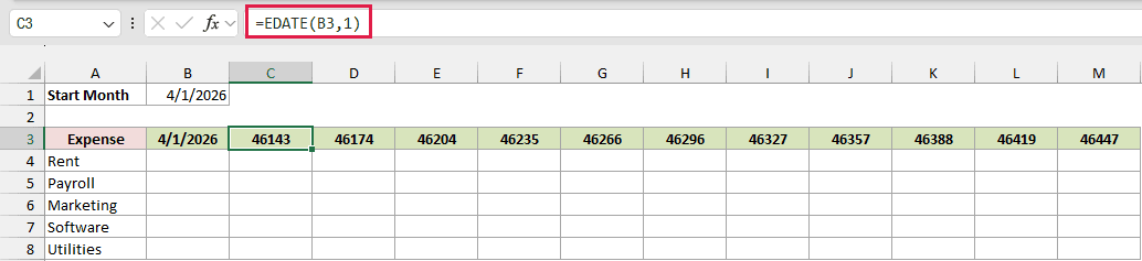
You’ll see 4/1/2026 in B3 and numbers such as 46143 in the other headers. With C3 selected, you can see its EDATE formula in the formula bar.
How does this formula work?
EDATE takes a date and a number of months, then returns the date that many months later. A negative number takes you back instead.
Here, EDATE(B3,1) returns the same day one month after B3. When you copy it to D3, the reference changes to EDATE(C3,1).
Each header therefore follows the one to its left. Because B3 points to B1, you control the whole row from that single start date.
Excel stores dates as numbers. The 46143 you see in C3 represents 1 May 2026, but you haven’t formatted that cell to display a month yet.
Here are the steps to display your headers as month and year:
- Select B3:M3 and press Ctrl + 1 to open the Format Cells dialog box.
- On the Number tab, click Custom in the Category list and type
mmm-yyin the Type box.
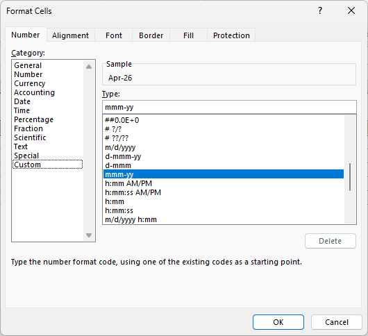
- Click OK.

Your headers now read Apr-26, May-26, Jun-26, and so on through Mar-27.
Change B1 to 1/1/2027, and every header updates to Jan-27 through Dec-27. You don’t need to retype any month names.

Method #2: Using SEQUENCE With EDATE
You can fill all 12 headers with one formula instead of copying EDATE across the row.
I recommend this method for Microsoft 365 or Excel 2021 and later. You enter the formula once, and changing your start date updates all 12 months.
Below, I have Rent, Payroll, Marketing, Software, and Utilities in A4:A8, with Expense in A3. You’ll fill B3:M3 with month headers above the empty expense cells.
Start Month is in A1, and B1 contains 4/1/2026. The header cells B3:M3 are empty, ready for the 12-month list.

Select B3:M3, press Ctrl + 1, pick Custom, and type mmm-yy.
Then enter this formula in B3 only:
=EDATE(B1,SEQUENCE(1,12,0))
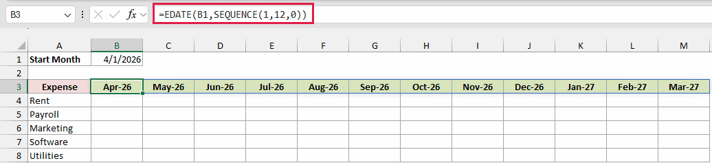
Your headers run from Apr-26 to Mar-27. With B3 selected, you can see the single formula that fills the entire row.
How does this formula work?
SEQUENCE(1,12,0) returns one row of 12 numbers, starting at 0: 0, 1, 2, and so on through 11.
EDATE adds each number of months to your start date in B1. Zero returns the start month, while 11 returns the month 11 months later.
The results fill B3:M3 automatically. This is called spilling, and you don’t need a separate formula in each header cell.
Change B1 to move all 12 headers forward or back. For a longer or shorter list, change the 12 in SEQUENCE to your preferred number of months.
Note: Keep C3:M3 empty before entering the formula. If a cell blocks the results, you’ll get a #SPILL! error.
Method #3: Using TODAY and EOMONTH (Last 12 Months)
To keep your report ending with the current month, you can replace the typed start date with a formula that follows today’s date.
You’ll get the last 12 months, including the current month, without maintaining a start cell. This is useful for a rolling 12-month report.
Below, I have Expense in A1 and Rent, Payroll, Marketing, Software, and Utilities in A2:A6. You’ll fill the empty B1:M1 headers above the expense planning cells.

In Microsoft 365 or Excel 2021 and later, format B1:M1 as mmm-yy and enter this formula in B1:
=EDATE(EOMONTH(TODAY(),-12)+1,SEQUENCE(1,12,0))

The screenshot was taken in October 2026, so the list in it runs from Nov-25 through Oct-26. B1 is selected to show the formula.
Open the file in November 2026, and you’ll see Dec-25 through Nov-26 instead.
Note: In Excel 2019 or earlier, put =EOMONTH(TODAY(),-12)+1 in B1 and =EDATE(B1,1) in C1, then copy C1 across to M1.
How does this formula work?
TODAY() returns today’s date, which is 12 October 2026 in the screenshot.
EOMONTH(TODAY(),-12) returns the last day of the month 12 months back: 31 October 2025. Adding 1 moves your start date to 1 November 2025.
EDATE then uses the numbers from SEQUENCE(1,12,0) to return that month and the next 11. Your final header is the current month.
Starting on the first day keeps every header on day 1. TODAY recalculates when you open or recalculate the workbook, so your window moves as the months change.
To show the last 12 complete months, ending with last month, change -12 to -13:
=EDATE(EOMONTH(TODAY(),-13)+1,SEQUENCE(1,12,0))
In October 2026, you’ll get Oct-25 through Sep-26. That keeps the unfinished current month out of your report.
Method #4: Using a Drop-Down List for the Start Month
For a template other people use, you can let them pick a month name instead of typing a date.
You’ll choose the start month from a drop-down and type the year below it. This also works for a fiscal year that starts in July.
First, create a sheet named Lists. Put Month in A1 and the three-letter month names, Jan through Dec, in A2:A13 in calendar order.
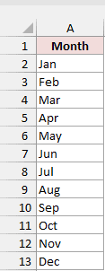
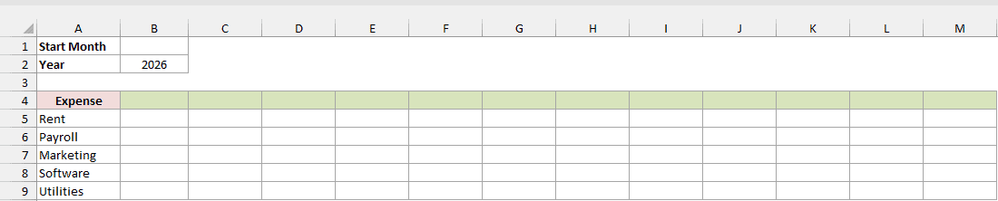
On your expense sheet, put Start Month in A1 and leave B1 empty for the drop-down. Put Year in A2 and 2026 in B2.
Below, I have Expense in A4 and Rent, Payroll, Marketing, Software, and Utilities in A5:A9. You’ll fill B4:M4 with headers above the empty expense planning cells.
Data Validation lets you restrict a cell to choices from a list. Here are the steps to make B1 your month selector:
- Select cell B1, then go to the Data tab and click Data Validation.
- On the Settings tab, choose List in the Allow drop-down and enter
=Lists!$A$2:$A$13in the Source box.
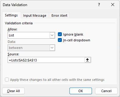
- Click OK.
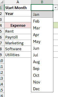
B1 now has a drop-down arrow when you select it. Click the arrow and pick Jul from the list.
In Microsoft 365 or Excel 2021 and later, format B4:M4 as mmm-yy, then enter this formula in B4:
=EDATE(DATE(B2,MATCH(B1,Lists!A2:A13,0),1),SEQUENCE(1,12,0))
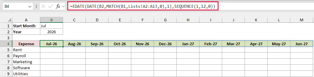
With Jul in B1 and 2026 in B2, your headers run from Jul-26 to Jun-27. B4 contains the formula for all 12 headers.
How does this formula work?
MATCH(B1,Lists!A2:A13,0) finds the chosen month’s position in your helper list. Jul is the seventh item, so MATCH returns 7.
DATE(B2,7,1) combines the year in B2 with month 7 and day 1. For this selection, it returns 1 July 2026.
EDATE uses SEQUENCE(1,12,0) to return that date and the next 11 months, just as in Method #2.
Pick a different month or change the year, and your headers roll with it. Picking Jan with 2026 in B2 returns Jan-26 through Dec-26.
For Excel 2019 or earlier, format B4:M4 as mmm-yy, enter the first formula in B4 and the second in C4, then copy C4 across to M4:
=DATE(B2,MATCH(B1,Lists!A2:A13,0),1)
=EDATE(B4,1)
How to Sum Data for Each Rolling Month
Once you have rolling months, you can use them to total dated orders with SUMIFS. I’ll build a six-month sales summary beside an order list.
Below, I have 12 orders in A1:C13, with Order ID, Order Date, and Amount as the headings. Your order dates run from 1/14/2026 to 7/11/2026.
Start Month is in E1, with 2/1/2026 in F1. Month and Total Sales are in E3:F3, ready for your monthly summary below.
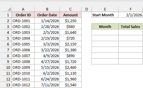
First, format E4:E9 as mmm-yy and enter this formula in E4 to list your months down the column:
=EDATE(F1,SEQUENCE(6,1,0))
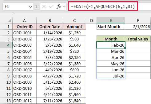
Your month column runs from Feb-26 to Jul-26. SEQUENCE(6,1,0) makes six rows instead of 12 columns.
Next, enter this formula in F4 and copy it down to F9.
Format F4:F9 as currency with 0 decimal places to display your sales totals:
=SUMIFS($C$2:$C$13,$B$2:$B$13,">="&E4,$B$2:$B$13,"<"&EDATE(E4,1))
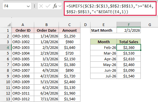
Your totals are $2,360 for February, $3,530 for March, $2,610 for April, $2,460 for May, $3,090 for June, and $1,540 for July.
How does this formula work?
SUMIFS adds the amounts in C2:C13 for orders that meet both date conditions. The dollar signs keep your source ranges fixed when you copy the formula down.
">="&E4 includes orders on or after your month’s first day. In F4, that’s 1 February 2026.
"<"&EDATE(E4,1) includes orders before the first day of the next month, 1 March 2026. You count the whole month regardless of its length.
Your two January orders, ORD-1001 and ORD-1002, are left out because January isn’t in this six-month window.
I put the formula in each row and copy it down to keep each month’s two date conditions easy to read.
Change F1 to 3/1/2026, and your summary runs from Mar-26 to Aug-26. August shows $0 because you don’t have any August orders yet.
Additional Notes About Rolling Months in Excel
Keep these date details in mind when you use rolling months in a budget or report:
- Chaining EDATE from 1/31/2026 gives 2/28/2026, then 3/28/2026. A month-only format hides the drift, so your SUMIFS date ranges end up off.
- Start on the first day of the month.
=EOMONTH(date,-1)+1turns any date into the first day of its month. - Keep your headers as real dates, formatted to display months. That lets you compare them with order dates in SUMIFS. For text, such as a chart title, use
=TEXT(B3,"mmm yyyy"). - TODAY is volatile, so your date-based window changes when the month changes and the workbook recalculates. For a frozen report, type a date and reference that cell instead.
- EDATE and EOMONTH need a single date or a single cell as the date argument. Range references such as B3:M3 or B3# return #VALUE!. With EDATE, put SEQUENCE in the months argument.
Frequently Asked Questions
Here are a few more ways you might want to create or display your month list.
Can I Make Rolling Months Without a Formula?
You can create a month list without a formula, but it won’t update when you change the first date.
Type the first date and drag the fill handle across. Then click the Auto Fill Options button and pick Fill Months.
You’ll get fixed dates. For headers that follow a changed start month, use one of the formula methods above.
How Do I Show Full Month Names Like April 2026?
Use the custom number format mmmm yyyy to display April 2026. For just April, use mmmm.
You’ll change how the date looks while keeping its underlying value available for calculations.
How Do I Create Rolling Quarter Headers?
With your start date in B1, use this formula to create four quarter headers:
=EDATE(B1,SEQUENCE(1,4,0,3))
SEQUENCE’s fourth argument, the step, is 3, so you get every third month.
With 4/1/2026 in B1, you’ll get Apr-26, Jul-26, Oct-26, and Jan-27. Format the output cells as mmm-yy.
How Do I Show the Next 12 Months Starting From the Current Month?
Use this formula to start on the first day of the current month and list that month plus the next 11:
=EDATE(EOMONTH(TODAY(),-1)+1,SEQUENCE(1,12,0))
In October 2026, you’ll get Oct-26 through Sep-27.
Conclusion
I’d use SEQUENCE with EDATE for most Microsoft 365 month lists, or the copied EDATE formula in an older version.
Use TODAY and EOMONTH when your months should follow today’s date, and the drop-down when other people need to pick a start month.
Other Excel articles you may also like:
