
If you need an inclusive percentile in Excel, PERCENTILE.INC is the current function name to use.
PERCENTILE is the older compatibility name, and both functions return the same answer.
In this article, I’ll show you how to read PERCENTILE.INC results, choose the right k values, and handle practical data issues.
PERCENTILE.INC normally returns one value for each k. In Excel 2021 and later, a range of k values can make it spill multiple results.
PERCENTILE.INC Function Syntax in Excel
The PERCENTILE.INC function uses a data array and an inclusive percentile value.
=PERCENTILE.INC(array, k)
- array (required) is the range or array of numeric data.
- k (required) is the percentile value from 0 to 1, including both endpoints.
When to Use PERCENTILE.INC Function
- Use Microsoft’s current function name instead of the older PERCENTILE compatibility name.
- Find an inclusive percentile when k may be 0 or 1.
- Calculate an interpolated cutoff that may not appear in the source data.
- Return several percentiles by supplying a range of k values.
- Calculate a percentile for one group by combining PERCENTILE.INC with FILTER.
Example 1: Why Results May Not Match the Data
Let’s start with the interpolation that often makes a correct result look suspicious.
Below is the dataset. Columns A and B list eight bakeries and loaves sold. In column D, you type k values 0.00, 0.25, 0.50, and 1.00.
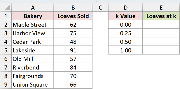
We want to see where all four k values land in the same set of loaf counts.
For the inclusive minimum, here is the formula:
=PERCENTILE.INC($B$2:$B$9,0)
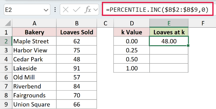
The result is 48.00, the smallest number in the range. PERCENTILE.INC accepts k = 0 because its endpoints are included.
For the 25th percentile, use this formula:
=PERCENTILE.INC($B$2:$B$9,0.25)
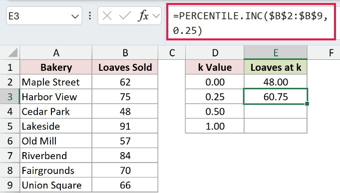
The result is 60.75, even though 60.75 does not appear in the source data.
With eight numbers, Excel calculates position 1 + 0.25 times 7, or 2.75. It moves three quarters of the way from 57 to 62.
For the median position, use k = 0.5:
=PERCENTILE.INC($B$2:$B$9,0.5)
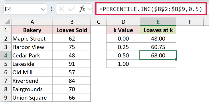
The result is 68.00, halfway between the fourth and fifth sorted values, 66 and 70.
For the inclusive maximum, here is the formula:
=PERCENTILE.INC($B$2:$B$9,1)
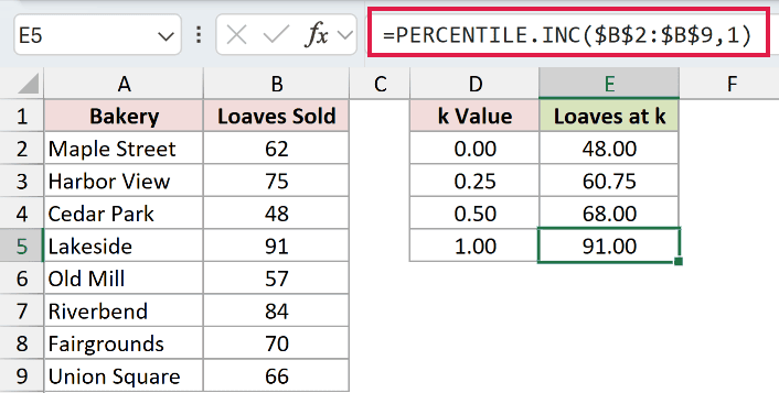
The result is 91.00, the largest number in the range. This is the other included endpoint.
Pro Tip: Interpolated results are calculated points between two sorted values when k does not land on a whole-number position, so they may not appear in the data.
Example 2: PERCENTILE.INC and PERCENTILE Match
The formulas in this example settle the naming question with results from real cells.
Below is the dataset. Columns A and B list 12 bike-share stations and their daily ride counts.
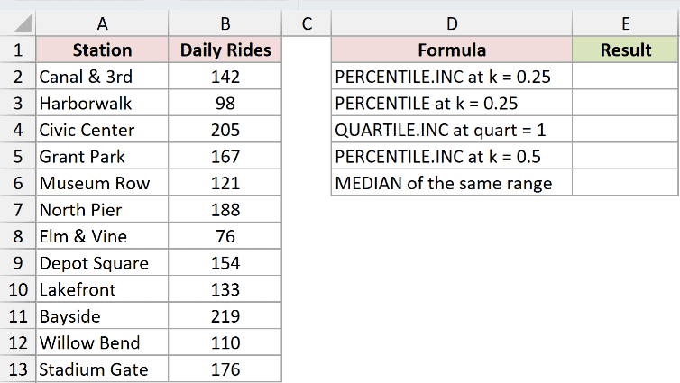
We want to compare the current name with its compatibility alias and two purpose-built equivalents.
First, here is PERCENTILE.INC at k = 0.25:
=PERCENTILE.INC($B$2:$B$13,0.25)
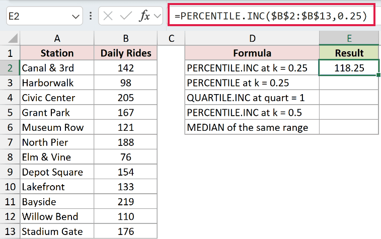
The result is 118.25.
Next, here is the older PERCENTILE name with the same range and k:
=PERCENTILE($B$2:$B$13,0.25)
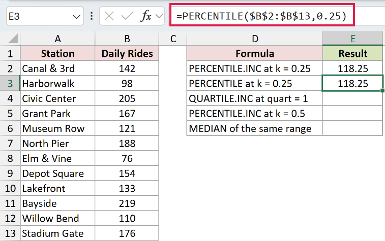
PERCENTILE also returns 118.25. Microsoft keeps this older name so existing workbooks continue to calculate, but warns that it may not be available in future Excel versions.
For a first quartile, QUARTILE.INC is the purpose-built equivalent:
=QUARTILE.INC($B$2:$B$13,1)
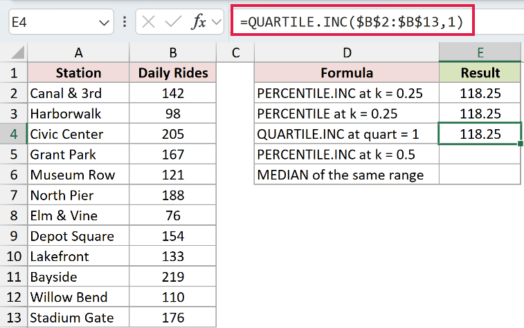
QUARTILE.INC returns 118.25 too because quart = 1 corresponds to k = 0.25.
Here is PERCENTILE.INC at k = 0.5:
=PERCENTILE.INC($B$2:$B$13,0.5)
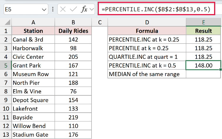
The result is 148.00.
For comparison, MEDIAN uses this shorter formula:
=MEDIAN($B$2:$B$13)
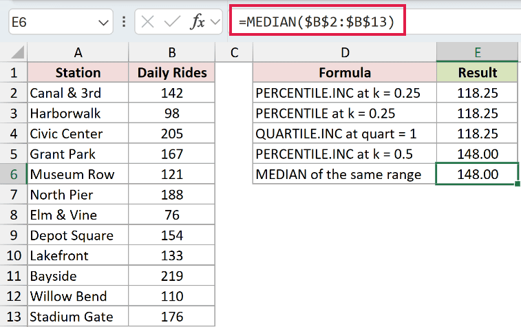
MEDIAN also returns 148.00 because the median is the 50th percentile.
For new workbooks, use PERCENTILE.INC. Keep PERCENTILE only when a file must remain compatible with Excel 2007 or earlier.
Example 3: Spill Multiple Percentiles From One Formula
Here’s the useful exception to the function’s usual single-result behavior.
Below is the dataset. Columns A and B list 12 connection IDs and download speeds. Column D contains five k values you type.
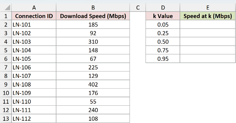
We want one formula to return a matching speed for every k value.
Here is the spilling formula:
=PERCENTILE.INC($B$2:$B$13,D2:D6)
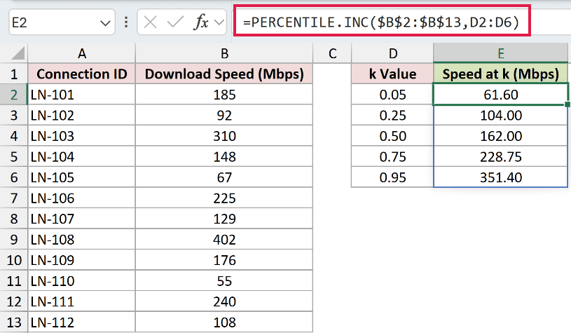
The formula returns 61.60, 104.00, 162.00, 228.75, and 351.40 beside k values 0.05 through 0.95.
PERCENTILE.INC still reduces the data range to one answer per k. The range in D2:D6 gives Excel five k values, so five answers spill.
Pro Tip: The data range still produces one answer per k. The D2:D6 k range expands the output, even though PERCENTILE.INC remains a reducer.
Example 4: Four k Values, One EXC Error
This example runs four k values side by side, showing exact agreement at 0.50 and a real #NUM! from PERCENTILE.EXC at 0.10.
Below is the dataset. Columns A and B list eight donors and donation amounts. Column D contains four k values you type.
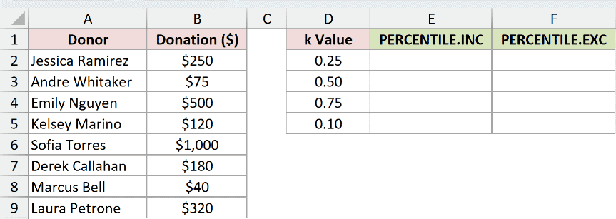
We want the inclusive percentile for each k value before comparing it with the exclusive definition.
Enter this formula in E2 and copy it down through E5:
=PERCENTILE.INC($B$2:$B$9,D2)
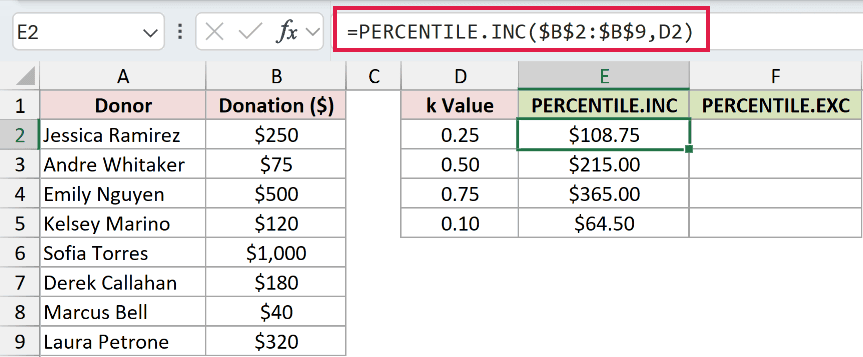
PERCENTILE.INC returns $108.75, $215.00, $365.00, and $64.50 for k values 0.25, 0.50, 0.75, and 0.10.
To compare the definitions, add this formula in F2 and copy it down. Use EXC only when you specifically need excluded endpoints.
=PERCENTILE.EXC($B$2:$B$9,D2)
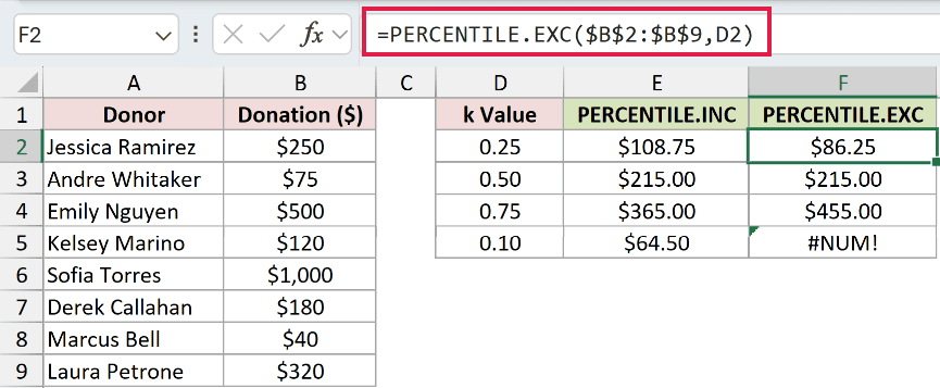
PERCENTILE.EXC returns $86.25, $215.00, $455.00, and #NUM! for those same four k values.
At k = 0.50, both definitions always return the same result, $215.00 here. Away from the middle, their different position rules produce different interpolated answers.
With eight numbers, PERCENTILE.EXC accepts k only from about 0.111 to 0.889. The final k of 0.10 falls outside that window, so Excel returns #NUM!.
PERCENTILE.INC includes 0 and 1, while PERCENTILE.EXC excludes those endpoints and can reject nearby values on small datasets.
Example 5: Ignore Blanks and Text in the Data
Now let’s see which cells Excel includes in the percentile calculation.
Below is the dataset. Columns A and B contain 12 weeks and rainfall readings, including one blank and one text entry. In column D, you type three k values.
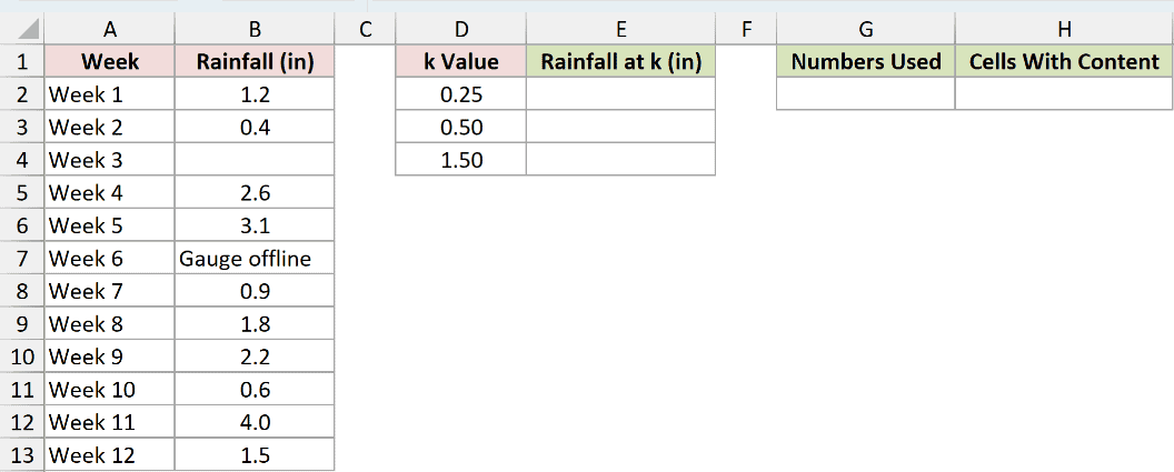
We want to calculate each percentile and confirm how many numeric readings Excel actually uses.
Enter this formula in E2 and copy it down through E4:
=PERCENTILE.INC($B$2:$B$13,D2)
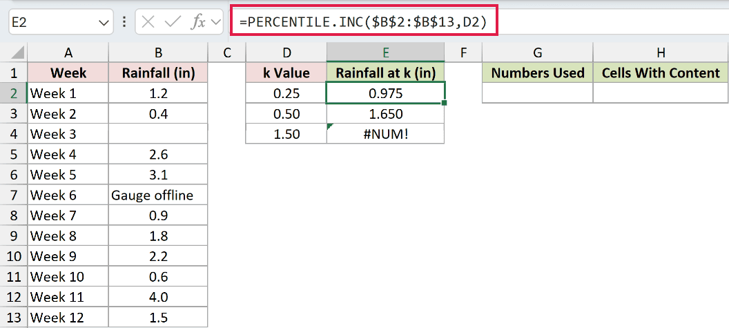
The formula returns 0.975 at k = 0.25 and 1.650 at k = 0.50. At k = 1.50, it returns #NUM!.
The blank and the text entry are ignored. The error occurs separately because k must stay between 0 and 1.
To count the numbers used across the entire Rainfall column, use:
=COUNT(B2:B13)
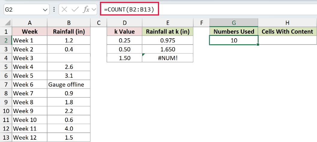
COUNT returns 10 because the column contains ten numeric readings.
To count every filled cell in that same column, use:
=COUNTA(B2:B13)
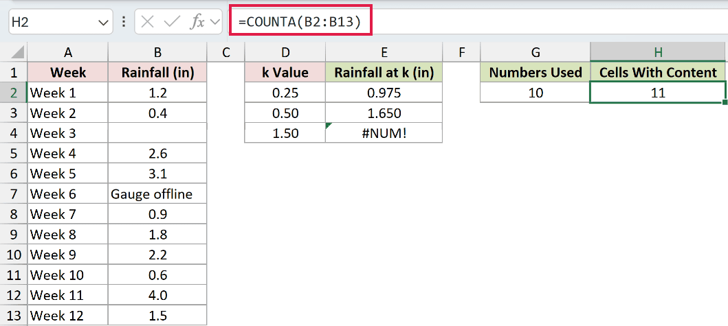
COUNTA returns 11 because it includes the ten numbers and the “Gauge offline” text cell.
These are sheet-level counts for the whole Rainfall column. They are not results for the k value shown on the same row.
Pro Tip: Enter k as a decimal from 0 to 1. A value such as 1.5 is outside the allowed range and returns #NUM!.
Example 6: Calculate Percentiles for Filtered Groups
Finally, let’s calculate separate percentiles from one mixed list.
Below is the dataset. Columns A through C list title IDs, formats, and last month’s checkouts. Column E contains the reader formats you type.
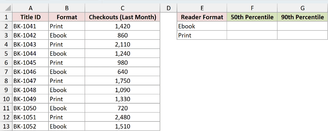
We want the 50th and 90th percentiles for Ebook and Print titles separately.
Enter this formula in F2 and copy it down to F3:
=PERCENTILE.INC(FILTER($C$2:$C$13,$B$2:$B$13=$E2),0.5)
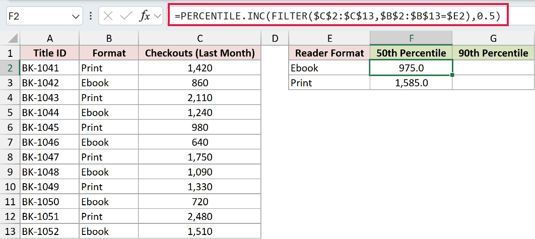
The 50th percentile is 975.0 for Ebook titles and 1,585.0 for Print titles.
FILTER keeps only rows whose format matches E2 or E3. PERCENTILE.INC then reduces each filtered set to one result.
For the 90th percentile, enter this formula in G2 and copy it down to G3:
=PERCENTILE.INC(FILTER($C$2:$C$13,$B$2:$B$13=$E2),0.9)
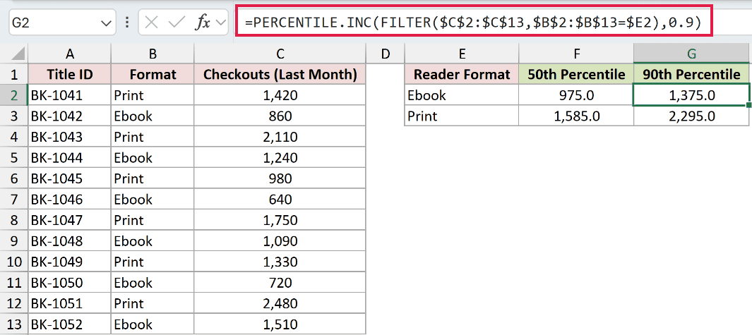
The 90th percentile is 1,375.0 for Ebook titles and 2,295.0 for Print titles.
FILTER creates each group, and PERCENTILE.INC reduces it to one cutoff.
Tips & Common Mistakes
- PERCENTILE.INC accepts k values from 0 to 1, including both endpoints. A value outside that range returns #NUM!.
- An empty array returns #NUM!, while a nonnumeric k returns #VALUE!.
- Blanks and text in the data array are ignored, so COUNT may reveal fewer observations than the visible row count suggests.
- PERCENTILE.INC is available in Excel 2010 and later.
- In Excel 2021 and later,
=PERCENTILE.INC(range,{0.05;0.25;0.5;0.75;0.95})spills five results vertically. - A spilled range reference also works as the data array. For example,
=PERCENTILE.INC(E2#,0.9)calculates a percentile from the values spilled from E2.
Use PERCENTILE.INC for new workbooks, and expect interpolated answers that may not appear in the source data.
If a result looks surprising, check k and count the numeric values before changing the formula.
Related Excel Functions / Articles:
